General sensitivity of rainfall to sea surface temperature (sst) changes in NINO region

Climate variability directly influences many aspects of food and nutrition security, particularly food availability and access. Variation in rainfall is a common element of many natural disasters – droughts, floods, typhoons and tsunamis – and is influenced by global, regional and/or local factors.

Global climate factors including El Niño, La Niña and the dipole mode; regional factors include monsoon circulation, the Madden-Julian oscillation and fluctuations in the surface temperature of the Indonesian Sea; and local factors can include elevation, island position, the circulation of land and sea breezes, and land cover.

The level of climate risk is measured based on the strength of ENSO signal on rainfall variability using correlation analysis. This approach is applied because production loss of food crops in Indonesia is closely associated with the ENSO phenomena. El Nino years is normally associated with drought years, while La-Nina is often related to wet years which can cause flood hazards. The correlation analysis is applied to monthly rainfall anomaly and sea surface temperature anomaly in NINO3.4.

The NINO-3.4 region is optimal for monitoring El Niño-Southern Oscillation (ENSO) and its impacts in Indonesia and possibly Southeast Asia. Then I would like to see the correlation between rainfall and SST by looking the change in rainfall with 1° increase in sea surface temperature (SST) of NINO-3.4 region, as a signal for moderate El Niño.

Method

For this analysis, I used monthly rainfall from CHIRPS - CHC UCSB: https://www.chc.ucsb.edu/data/chirps and SST anomaly from ERSST v4 - NOAA: https://www.ncdc.noaa.gov/teleconnections/enso/indicators/sst/ for year 1981 - 2017. Rainfall data available in GeoTIFF, but SST is in text format. In order to do pixel-wise regression between two rasters, both data must available in GeoTIFF raster format and in the same dimension (width and height).

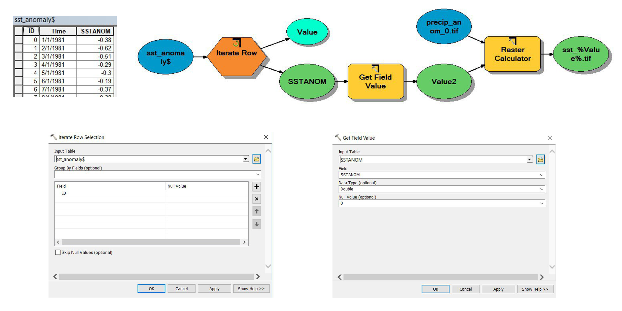
As the SST data is only from single location in NINO3.4 then I need to do some data tweak (I used ArcGIS Model Builder to create SST anomaly raster):

Prepare list of SST anomaly data from above link and save as Excel (*.xls) file, and add ID as first column.
Add Iterate Row Selection to Model Builder, choose sst_anomaly.xls as Input Table and ID as field.
Add Get Field Value from Model Only Tools within the Model Builder, add SSTANOM asInput Table and SSTANOM column as Field.
Add 1 of rainfall raster as example and will use this data as a template for SST to generate new raster with same dimension as rainfall.
By using Raster Calculator toolbox, and add
(precip_anom_0.tif / precip_anom_0.tif) * Value2
and give name sst_%Value%.tif as output raster.

Figure 1. Model Builder for generating SST raster — **Figure 1.** Model Builder for generating SST raster

Time series regression will apply to indicate the correlation between rainfall anomaly in each area to anomaly of SST in the Pacific Ocean which represent ENSO signals. And doing a pixel-wise regression between two raster time series can be useful for several reasons, for example:

Find the relation between vegetation and rainfall for each pixel, e.g. a low correlation could be a sign of degradation.
Derive regression coefficients to model depending variable using the independent variable (e.g. SST with rainfall data)

Using R Statistics, it is easy and fast to do pixel-wise time series regression between rainfall and sea surface temperature. Then put everything in one single stack and derive rasters showing the slope, intercept and R² of the two time series as pixel values:

# Define stacks in folder
rainanom_ <- paste0( '~/R/PWR/tls_rainanom/rainanom_' , 0 : 443 , ".tif" )
rainanom <- stack(rainanom_)
sstanom_ <- paste0( '~/R/PWR/tls_sstanom/sstanom_' , 0 : 443 , ".tif" )
sstanom <- stack(sstanom_)
s <- stack(rainanom, sstanom)
a <- length(rainanom_)
b <- length(sstanom_)

Then calculate the slope using below function

# Slope Function
fun <- function (x) { if (is.na(x[ 1 ]))   else {cochrane.orcutt(lm(x[ 1 :a] ~ x[( 1 +a):(a+b)]))$coefficients[ 2 ] }}
slope <- calc(s, fun)

Figure 2. Slope map — **Figure 2.** Slope map

Slope map above shows the changes in monthly rainfall likely to result from a 1°C change in sea surface temperature (SST). Areas in white exhibit very high negative change in rainfall: those in light to dark green exhibit very low negative changes to normal. Each square in the grid represents a 5.6 x 5.6 km square.

For correlation and p-value, we can used Gridded Correlation of Time Series Raster Data that available in Hakim Abdi's Github Gist: https://gist.github.com/hakimabdi/7308bbd6d9d94cf0a1b8

Figure 3. Correlation and p-value map — **Figure 3.** Correlation and p-value map

Timor-Leste data was used to test the script, and its worked. So we can apply it using data from other areas or with bigger dimension.

Reference:

Notes:

I completed data manipulation process for SST using ArcGIS Model Builder in 4 Dec 2018, after got feedback and insight from discussion in GIS ID Telegram group.
This works done by Anggita Annisa, a final year student from Department of Statistics - IPB who is doing an internship under my supervision in VAM unit of WFP Indonesia from June - August 2019.

Update - 17 May 2020

Data and script: https://github.com/wfpidn/Pixel-wise-Regression

Pixel-wise regression between rainfall and sea surface temperature

Technical engagement workshop in Beijing

Summer in Mongolia