Fuzzy Inference System (FIS) for Flood Risk Assessment
1 Implementation
In the implementation phase of this analysis, we utilized Python and the Scikit-Fuzzy library to develop a fuzzy logic-based flood risk assessment model. This model took into account four essential factors affecting flood risks: precipitation intensity, soil moisture, land cover, and slope. By defining the fuzzy sets and rules for these variables, the model was able to estimate the flood risk for various combinations of input values. The ultimate goal of this implementation was to identify the conditions under which low flood risks could be achieved, even in situations where precipitation intensity was at its maximum.
# Install packages
!pip install numpy scipy matplotlib scikit-fuzzy seaborn pandas

# Import the packages
import numpy as np
import skfuzzy as fuzz
from skfuzzy import control as ctrl
import matplotlib.pyplot as plt
import matplotlib.patches as mpatches
import mpl_toolkits.mplot3d
from mpl_toolkits.mplot3d import Axes3D
from scipy.optimize import minimize
import seaborn as sns
import pandas as pd
1.1 How-to?
In the first stage of the analysis, we defined the variables that influence flood risk. These variables include precipitation intensity, soil moisture, land cover, and slope. Each of these variables was represented as a fuzzy variable using the Scikit-Fuzzy library's Antecedent class. Additionally, we defined the output variable flood_risk using the Consequent class. This stage set the foundation for the fuzzy logic-based flood risk assessment model by establishing the key variables that the model would use to estimate flood risk.
# Stage 1:
# Define the variables
precipitation = ctrl.Antecedent(np.arange(0, 101, 1), 'precipitation')
soil_moisture = ctrl.Antecedent(np.arange(0, 101, 1), 'soil_moisture')
land_cover = ctrl.Antecedent(np.arange(0, 101, 1), 'land_cover')
slope = ctrl.Antecedent(np.arange(0, 91, 1), 'slope')
flood_risk = ctrl.Consequent(np.arange(0, 101, 1), 'flood_risk')

# Define the output variable
flood_risk = ctrl.Consequent(np.arange(0, 101, 1), 'flood_risk')
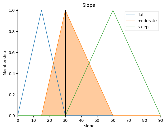
In the second and third stages, we focused on defining the fuzzy sets and their respective membership functions for each of the variables defined in the first stage. We used the automf() function to automatically generate triangular membership functions for precipitation intensity, soil moisture, and flood risk, each with three levels: low, medium, and high. For the land cover and slope variables, we manually defined triangular membership functions, specifying the appropriate ranges for each fuzzy set (urban, vegetation, and bare_soil for land cover, and flat, moderate, and steep for slope). These stages were critical for establishing the relationships between the input variables and the output flood risk, which would later be used to evaluate different combinations of input values in the fuzzy inference process.
# Stage 2 & 3:
# Define the fuzzy sets and their membership functions
precipitation.automf(3, names=['low', 'medium', 'high'])
soil_moisture.automf(3, names=['low', 'medium', 'high'])
land_cover['urban'] = fuzz.trimf(land_cover.universe, [0, 25, 50])
land_cover['vegetation'] = fuzz.trimf(land_cover.universe, [25, 50, 75])
land_cover['bare_soil'] = fuzz.trimf(land_cover.universe, [50, 75, 100])
slope['flat'] = fuzz.trimf(slope.universe, [0, 15, 30])
slope['moderate'] = fuzz.trimf(slope.universe, [15, 30, 60])
slope['steep'] = fuzz.trimf(slope.universe, [30, 60, 90])
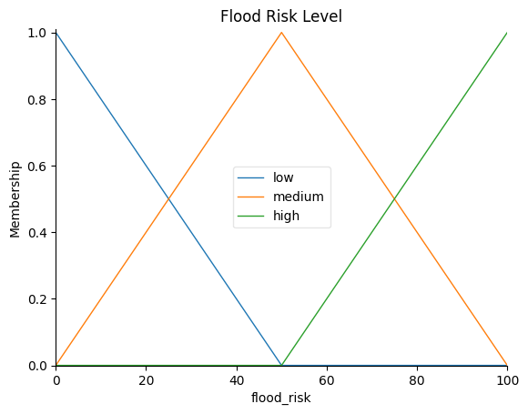
flood_risk.automf(3, names=['low', 'medium', 'high'])
flood_risk['very_low'] = fuzz.trimf(flood_risk.universe, [0, 0, 10])
In the fourth stage, we defined the rules that describe the relationships between the input variables (precipitation intensity, soil moisture, land cover, and slope) and the output variable (flood risk). We first created a list of classifications for each input variable and the output variable. Using the multiplication principle, we calculated the total number of possible combinations of these classifications, resulting in 81 unique rules.
For each combination of input classifications, we determined the appropriate flood risk level based on a set of predefined conditions. These conditions were based on expert knowledge and domain understanding, considering factors such as high precipitation and soil moisture, bare soil land cover, and steep slopes. After determining the flood risk level for each combination, we created a fuzzy rule using the Scikit-Fuzzy library's Rule class, linking the input conditions with the corresponding flood risk level. These rules formed the basis of the fuzzy inference system that was used to evaluate different scenarios and estimate the corresponding flood risks.
# Stage 4:
# Define the rules
precipitation_levels = ['low', 'medium', 'high']
soil_moisture_levels = ['low', 'medium', 'high']
land_cover_types = ['urban', 'vegetation', 'bare_soil']
slope_levels = ['flat', 'moderate', 'steep']
flood_risk_levels = ['low', 'medium', 'high']

# We can use the multiplication principle to calculate the total number of combinations.
# If we have n variables and each variable can take on one of m classifications,
# then the total number of combinations is m^n, total rules for this case will be 3^4 = 81 rules

rules = []

for p_level in precipitation_levels:
    for sm_level in soil_moisture_levels:
        for lc_type in land_cover_types:
            for s_level in slope_levels:
                # Determine the appropriate flood risk level based on the input conditions
                if p_level == 'high' and sm_level == 'high' and lc_type == 'bare_soil' and s_level == 'steep':
                    fr_level = 'high'
                elif p_level == 'medium' and sm_level == 'medium' and lc_type == 'bare_soil' and s_level == 'steep':
                    fr_level = 'high'
                elif p_level == 'high' and sm_level == 'high' and s_level != 'flat':
                    fr_level = 'high'
                elif p_level == 'high' and sm_level == 'medium' and s_level != 'flat':
                    fr_level = 'high'
                elif p_level == 'high' and lc_type == 'bare_soil' and s_level != 'flat':
                    fr_level = 'high'
                elif p_level == 'medium' and sm_level == 'medium' and lc_type == 'bare_soil' and s_level != 'flat':
                    fr_level = 'high'
                elif p_level == 'medium' and sm_level == 'high' and s_level != 'flat':
                    fr_level = 'high'
                elif p_level == 'medium' and s_level == 'steep':
                    fr_level = 'high'
                elif p_level == 'high' and s_level != 'flat':
                    fr_level = 'high'
                elif p_level == 'high' and sm_level == 'low':
                    fr_level = 'medium'
                elif p_level == 'medium' and sm_level == 'low' and s_level == 'steep':
                    fr_level = 'medium'
                else:
                    fr_level = 'low'

                # Create the rule with the determined conditions and consequences
                rule = ctrl.Rule(
                    precipitation[p_level] & soil_moisture[sm_level] & land_cover[lc_type] & slope[s_level],
                    flood_risk[fr_level]
                )
                rules.append(rule)

                # This catch_all_rule will activate the 'very_low' flood risk when no other rules are fired.
                # It uses the negation operator ~ to ensure that this rule is activated only when none of
                # the other input fuzzy sets are activated.
                catch_all_rule = ctrl.Rule(antecedent=(~precipitation['high'] & ~precipitation['medium'] & ~precipitation['low'] &
                                                      ~soil_moisture['high'] & ~soil_moisture['medium'] & ~soil_moisture['low'] &
                                                      ~land_cover['urban'] & ~land_cover['vegetation'] & ~land_cover['bare_soil'] &
                                                      ~slope['flat'] & ~slope['moderate'] & ~slope['steep']),
                                          consequent=flood_risk['very_low'])

                rules.append(catch_all_rule)
In the fifth stage, we created the control system and simulation by combining the defined rules from the previous stage. The Scikit-Fuzzy library's ControlSystem and ControlSystemSimulation classes were used for this purpose. The ControlSystem class takes the set of rules as input and initializes the fuzzy inference system, while the ControlSystemSimulation class initializes a simulation environment that can be used to compute the output based on the input values.
# Stage 5:
# Create the control system and simulation
flood_risk_ctrl = ctrl.ControlSystem(rules)
flood_risk_sim = ctrl.ControlSystemSimulation(flood_risk_ctrl)
In the sixth stage, we provided example input values for each input variable (precipitation, soil moisture, land cover, and slope) to test the fuzzy inference system. The input values were assigned to their corresponding input variables in the simulation, and the compute method of the ControlSystemSimulation object was called to perform the fuzzy inference process and obtain the output flood risk level.
# Stage 6:
# Input example values and compute the output
precipitation_value = 100
soil_moisture_value = 50
land_cover_value = 25
slope_value = 30

flood_risk_sim.input['precipitation'] = precipitation_value
flood_risk_sim.input['soil_moisture'] = soil_moisture_value
flood_risk_sim.input['land_cover'] = land_cover_value
flood_risk_sim.input['slope'] = slope_value

flood_risk_sim.compute()
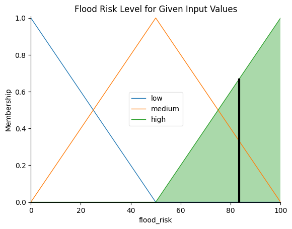
In the final stage, we output the computed flood risk level and visualize the result using the Scikit-Fuzzy library's built-in plotting capabilities. The flood risk level was displayed as a numerical value, while the visualization provided a graphical representation of the membership functions and the defuzzified output. This allowed us to assess the performance of the fuzzy inference system and analyze the relationships between the input variables and the flood risk.
# Stage 7:
# Define the flood risk category
def categorize_flood_risk(flood_risk_value):
    if flood_risk_value < 34:
        return "low"
    elif flood_risk_value < 67:
        return "medium"
    else:
        return "high"

# Output the result
flood_risk_value = flood_risk_sim.output['flood_risk']
flood_risk_category = categorize_flood_risk(flood_risk_value)
print("Flood Risk Value:", flood_risk_value)
print("Flood Risk Category:", flood_risk_category)

# Update the membership function values
flood_risk['low'].mf = flood_risk['low'].mf
flood_risk['medium'].mf = flood_risk['medium'].mf
flood_risk['high'].mf = flood_risk['high'].mf

# Remove the 'very_low' term
if 'very_low' in flood_risk.terms:
    del flood_risk.terms['very_low']

# Plot the result without the 'very_low' term
flood_risk.view(sim=flood_risk_sim)
This will returned:
Flood Risk Value: 83.33333333333336
Flood Risk Category: high
And a plot below
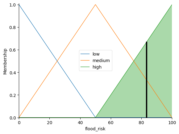
The initial implementation of the fuzzy inference system for flood risk assessment has been completed successfully. By providing example input values for precipitation (100), soil moisture (50), land cover (25), and slope (30) in Stage 6, we have demonstrated the functionality of the fuzzy system. The system processes these inputs through the defined membership functions, rules, and defuzzification methods to produce an output flood risk value and the corresponding flood risk category.
Upon evaluating the system with the given input values, a flood risk value is generated, and the flood_risk.view(sim=flood_risk_sim) function provides a visual representation of the output. The plot displays the aggregated output membership functions and indicates the defuzzified crisp value. In this case, the plot reflects the flood risk level based on the provided inputs, and the computed flood risk category helps to understand the risk associated with the given conditions. With this initial implementation, we have set the foundation for further analyses and can adapt or extend the fuzzy system as needed to address specific flood risk assessment scenarios.
1.2 Plot the membership function of the input variables
The provided code visualizes the membership functions for each of the input variables (Precipitation Intensity, Soil Moisture, Land Cover, and Slope) and the output variable (Flood Risk Level) in the fuzzy inference system. Here's a summary of what each part of the code does:
precipitation.view(sim=flood_risk_sim): Plots the membership functions for the Precipitation Intensity variable, displaying how the input values are categorized into low, medium, and high precipitation levels.soil_moisture.view(sim=flood_risk_sim): Plots the membership functions for the Soil Moisture variable, showing how the input values are categorized into low, medium, and high soil moisture levels.land_cover.view(sim=flood_risk_sim): Plots the membership functions for the Land Cover variable, illustrating how the input values are categorized into low, medium, and high land cover levels.slope.view(sim=flood_risk_sim): Plots the membership functions for the Slope variable, demonstrating how the input values are categorized into low, medium, and high slope levels.flood_risk.view(): Plots the membership functions for the output variable, Flood Risk Level, indicating how the output values are categorized into low, medium, and high flood risk levels.flood_risk.view(sim=flood_risk_sim): Plots the final Flood Risk Level for given input values, illustrating how the fuzzy inference system computes the flood risk based on the input variable values and the defined fuzzy rules.
# Plot the membership functions of the input variables
precipitation.view(sim=flood_risk_sim)
plt.title("Precipitation Intensity")
plt.show()

soil_moisture.view(sim=flood_risk_sim)
plt.title("Soil Moisture")
plt.show()

land_cover.view(sim=flood_risk_sim)
plt.title("Land Cover")
plt.show()

slope.view(sim=flood_risk_sim)
plt.title("Slope")
plt.show()

# Plot the membership functions of the output variable
flood_risk.view()
plt.title("Flood Risk Level")
plt.show()

# Plot the final output (flood risk) given the input values
flood_risk.view(sim=flood_risk_sim)
plt.title("Flood Risk Level for Given Input Values")
plt.show()
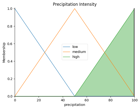
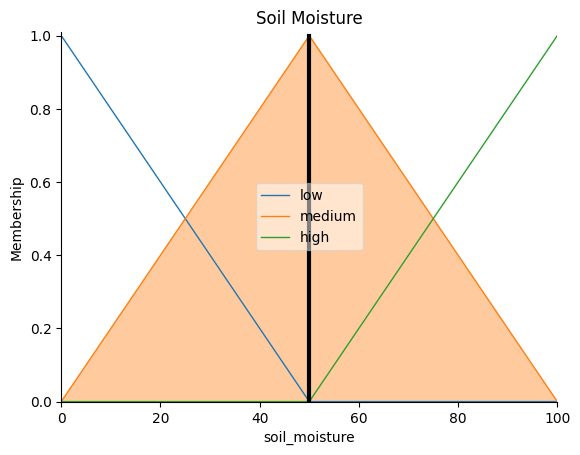
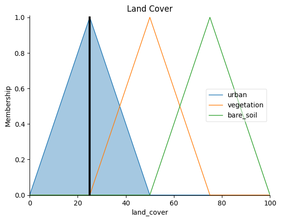
To interpret the plots, observe how each input variable is divided into categories (low, medium, high) based on the membership functions. These categories represent the degree to which an input value belongs to a particular category.
The output variable plot shows how the flood risk levels are determined based on the input variables' membership values and the fuzzy rules defined in the system. The final plot, Flood Risk Level for Given Input Values, displays the aggregated output membership functions and the computed flood risk level as a single value.
1.3 2D Plot
The provided code generates a 2D contour plot of flood risk as a function of Precipitation Intensity and Land Cover, while fixing the values of Soil Moisture and Slope. Here's a summary of what each part of the code does:
Create grid points for input variables: Define a range of values for each input variable (Precipitation Intensity, Soil Moisture, Land Cover, and Slope) using
np.linspace().Define
compute_flood_risk()function: This function takes Precipitation Intensity (P), Soil Moisture (M), Land Cover (L), and Slope (S) as inputs and computes the flood risk using the fuzzy inference system (flood_risk_sim).Fix Soil Moisture and Slope values: Assign fixed values to Soil Moisture (M_fixed) and Slope (S_fixed).
Create flood risk matrix: Initialize a matrix with the size of the combination of Precipitation Intensity (P_values) and Land Cover (L_values). Iterate through each combination of these values and compute the flood risk using the
compute_flood_risk()function with the fixed values of Soil Moisture and Slope.Plot the 2D contour plot: Using
plt.contourf(), create a contour plot that visualizes the flood risk as a function of Precipitation Intensity and Land Cover. The color map 'viridis' is used to represent the flood risk levels, with 20 contour levels.Add colorbar, labels, and title: Add a colorbar to represent the flood risk values, label the axes, and add a title that includes the fixed values of Soil Moisture and Slope.
# 2D plot
# Generate grid points for input variables
P_values = np.linspace(0, 200, 100)
M_values = np.linspace(0, 100, 100)
L_values = np.linspace(0, 100, 100)
S_values = np.linspace(0, 90, 100)

# Define a function to compute flood risk given input values
def compute_flood_risk(P, M, L, S):
    flood_risk_sim.input['precipitation'] = P
    flood_risk_sim.input['soil_moisture'] = M
    flood_risk_sim.input['land_cover'] = L
    flood_risk_sim.input['slope'] = S
    try:
        flood_risk_sim.compute()
        return flood_risk_sim.output['flood_risk']
    except ValueError:
        # Return the lowest possible flood risk if the system cannot compute a valid output
        return 0

# Fix two of the input variables at specific values
M_fixed = 50
S_fixed = 45

# Create flood risk matrix for different combinations of input variables
flood_risk_matrix = np.zeros((len(P_values), len(L_values)))

for i, P in enumerate(P_values):
    for j, L in enumerate(L_values):
        flood_risk_matrix[i, j] = compute_flood_risk(P, M_fixed, L, S_fixed)

# Plot the 2D contour plot for Precipitation vs Land Cover
X, Y = np.meshgrid(L_values, P_values)
plt.contourf(X, Y, flood_risk_matrix, cmap='viridis', levels=20)
plt.colorbar(label='Flood Risk')
plt.xlabel('Land Cover')
plt.ylabel('Precipitation Intensity')
plt.title(f'Flood Risk (Soil Moisture = {M_fixed}, Slope = {S_fixed})')
plt.show()

To interpret the plot, observe how the flood risk values change as the Precipitation Intensity and Land Cover values vary. The plot shows how the flood risk is influenced by these two input variables while keeping the other two (Soil Moisture and Slope) fixed at specific values.
The contour lines in the plot represent different levels of flood risk, with the color intensity indicating the flood risk level. Darker colors represent lower flood risk, and lighter colors represent higher flood risk.
1.4 3D Plot
The provided code generates a 3D surface plot of flood risk as a function of Precipitation Intensity and Land Cover, while fixing the values of Soil Moisture and Slope. Here's a summary of what each part of the code does:
Create a 3D plot figure: Initialize a new figure using
plt.figure()and add a 3D subplot with theprojection='3d'argument.Create the 3D surface plot: Use the
ax.plot_surface()function to create a 3D surface plot for Precipitation Intensity (Y-axis) vs Land Cover (X-axis), with the flood risk as the Z-axis. The color map 'viridis' is used to represent the flood risk levels.Add colorbar, labels, and title: Add a colorbar to represent the flood risk values, label the axes, and add a title that includes the fixed values of Soil Moisture and Slope.
# 3D plot
fig = plt.figure()
ax = fig.add_subplot(111, projection='3d')

# Create the 3D surface plot for Precipitation vs Land Cover
X, Y = np.meshgrid(L_values, P_values)
surf = ax.plot_surface(X, Y, flood_risk_matrix, cmap='viridis', linewidth=0, antialiased=False)

fig.colorbar(surf, shrink=0.5, aspect=5, label='Flood Risk')

ax.set_xlabel('Land Cover')
ax.set_ylabel('Precipitation Intensity')
ax.set_zlabel('Flood Risk')
ax.set_title(f'Flood Risk (Soil Moisture = {M_fixed}, Slope = {S_fixed})')

plt.show()
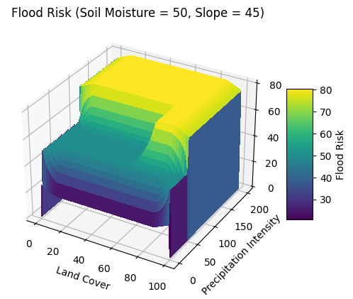
To interpret the plot, observe how the flood risk values (Z-axis) change as the Precipitation Intensity and Land Cover values (X and Y axes) vary. The plot shows how the flood risk is influenced by these two input variables while keeping the other two (Soil Moisture and Slope) fixed at specific values. The color intensity on the surface indicates the flood risk level, with darker colors representing lower flood risk and lighter colors representing higher flood risk.
The 3D surface plot provides a more detailed visualization of the relationship between flood risk, Precipitation Intensity, and Land Cover compared to the 2D contour plot. You can observe the shape of the surface to identify areas with high or low flood risk and better understand the interaction between the input variables.
2 Minimizing Flood Risks under Maximum Precipitation
This chapter emphasizes the focus on reducing flood risks under the most challenging conditions (maximum precipitation) while highlighting the three main variables (soil moisture, land cover, and slope) being examined in the analysis.
Flood risk management is a critical aspect of urban planning and environmental protection. Understanding the factors that contribute to flood risks and identifying strategies to minimize these risks is essential for creating resilient communities. In this analysis, we explore the relationships between four key variables - precipitation intensity, soil moisture, land cover, and slope - to determine their influence on flood risk. Our goal is to identify the combinations of these variables that result in low flood risks, even under conditions of maximum precipitation.
Using a fuzzy logic-based simulation model, we examine the interactions between these variables and their impact on flood risk. The model incorporates expert knowledge and rule-based systems to predict flood risk levels based on various input scenarios. By analyzing the simulation results, we aim to provide insights into the conditions that can effectively mitigate flood risks, helping policymakers and urban planners make informed decisions for better flood management strategies.
The analysis includes a scatterplot matrix visualization that highlights the relationships between soil moisture, land cover, and slope under maximum precipitation conditions. By interpreting this matrix, we can identify patterns and correlations between these variables that contribute to lower flood risks. These insights will help guide future efforts in designing urban areas and implementing flood management measures that are both effective and sustainable.
The provided code performs a sensitivity analysis to minimize flood risks under maximum precipitation conditions. It evaluates flood risk categories based on all input variables, generates a dataset of data points with different combinations of soil moisture, land cover, and slope values, and finally creates a scatterplot matrix. Here's a summary of what each part of the code does:
Define the maximum precipitation intensity: Set the value of
max_precipitationto 100, which is considered high precipitation intensity.Define the flood risk category function: Create a function
get_flood_risk_category()that takes precipitation, soil moisture, land cover, and slope as input variables, and returns the flood risk category using the previously definedcategorize_flood_risk()function.Generate data points for soil moisture, land cover, and slope: Create arrays of evenly spaced values for each of these input variables.
Iterate through all combinations of soil moisture, land cover, and slope: For each combination, use the maximum precipitation value and the
get_flood_risk_category()function to obtain the flood risk category. If the category is notNone, append the combination to thedata_pointslist.Create a DataFrame containing the data points: Convert the list of data points into a pandas DataFrame, which makes it easier to analyze and visualize the data.
Create a scatterplot matrix: Use the seaborn library's
pairplot()function to create a scatterplot matrix of the data points, with flood risk categories represented by different colors.
# Maximum value to be used to define as high precipitation intensity
max_precipitation = 100

# Define the flood risk category based on all variables
def get_flood_risk_category(precipitation, soil_moisture, land_cover, slope):
    flood_risk_sim.input['precipitation'] = precipitation
    flood_risk_sim.input['soil_moisture'] = soil_moisture
    flood_risk_sim.input['land_cover'] = land_cover
    flood_risk_sim.input['slope'] = slope

    try:
        flood_risk_sim.compute()
        flood_risk_value = flood_risk_sim.output['flood_risk']
        return categorize_flood_risk(flood_risk_value)
    except ValueError:
        return None

# Generate data points for soil moisture, land cover, and slope
soil_moisture_values = np.linspace(0, 100, num=20)
land_cover_values = np.linspace(0, 100, num=20)
slope_values = np.linspace(0, 90, num=20)

data_points = []

# Iterate through all combinations of soil moisture, land cover, and slope
for soil_moisture in soil_moisture_values:
    for land_cover in land_cover_values:
        for slope in slope_values:
            category = get_flood_risk_category(max_precipitation, soil_moisture, land_cover, slope)
            if category is not None:
                data_points.append({
                    'Soil Moisture': soil_moisture,
                    'Land Cover': land_cover,
                    'Slope': slope,
                    'Flood Risk Category': category
                })

# Create a DataFrame containing the data points
data = pd.DataFrame(data_points)

# Create a scatterplot matrix
sns.pairplot(data, hue='Flood Risk Category', markers='o', diag_kind='hist')
plt.show()

Here's how to read the scatterplot matrix:
The diagonal plots (from the top-left to the bottom-right) are bar plots showing the distribution of each variable. These plots give an idea of the frequency of different values for each variable when the flood risk is low under maximum precipitation conditions.
The off-diagonal plots are scatter plots showing the relationships between pairs of variables. These plots help identify any patterns or correlations between the variables. The color of the dots indicates the flood risk category associated with each data point.
In the off-diagonal plots, if you see that dots of a specific color (in this case, low flood risk) are clustered in a particular region, it indicates that certain combinations of variables are more likely to result in low flood risk conditions.
To interpret the plots, consider the following:
In the scatterplot between soil moisture and land cover, if there is a pattern or a specific region where low flood risk dots are clustered, it would suggest that there's a relationship between these two variables that contributes to lower flood risks under maximum precipitation conditions.
Similarly, in the scatterplot between soil moisture and slope, look for clusters or patterns of low flood risk dots to identify any relationships between these variables that contribute to lower flood risks.
Finally, in the scatterplot between land cover and slope, examine the distribution of low flood risk dots to determine if there's a connection between these variables that leads to lower flood risks.
By analyzing these plots, we can gain insights into the relationships between soil moisture, land cover, and slope that contribute to low flood risks even under maximum precipitation conditions.
3 Sensitivity Analysis
After obtaining the flood risk assessment results from the Fuzzy Inference System (FIS), we can assess the quality of the model by comparing its predictions to observed data. To do this, we'll need a dataset containing historical flood events along with the corresponding values of the input variables (Precipitation Intensity, Soil Moisture, Land Cover, and Slope).
What if observation data on flood events never exist?
If we don't have any observation data to compare the FIS model results, evaluating the model's performance becomes more challenging. However, we can still follow some steps to ensure that your FIS model is reasonable and plausible:
Expert knowledge: Consult with experts in the field of flood risk assessment to ensure that your fuzzy sets, membership functions, and fuzzy rules are realistic and based on sound principles. This can help us refine our FIS model even without actual observation data.
Sensitivity analysis: Perform a sensitivity analysis to understand how the output flood risk varies with changes in input variables. By altering the input variables within their expected range and studying the corresponding changes in flood risk, we can gain insight into the behavior of the model and identify any unrealistic responses.
Comparison with other models: If there are other flood risk assessment models available (either deterministic or statistical), compare your FIS model's predictions with those from the other models. Although this is not a direct comparison with observed data, it can provide some indication of how your model's performance compares to alternative approaches.
Simulation data: If we have access to hydrological or hydraulic models that can simulate flood events, we can use the simulated data as a proxy for observed data. Although this approach has its limitations, as the simulated data may not perfectly represent real-world conditions, it can still provide valuable information for evaluating your FIS model.
Temporal validation: If we have historical data for some of the input variables but not for the flood risk, we can still evaluate your FIS model by analyzing its performance over time. For instance, we can assess whether the model's predictions of high flood risk align with periods of heavy rainfall, high soil moisture, or other conditions known to increase flood risk.
Remember that without observed data, it is more challenging to assess the performance of your FIS model accurately. However, following the steps outlined above can help us gain some confidence in your model and identify areas for potential improvement.
Let’s try Sensitivity Analysis
We'll use the One-at-a-time (OAT) sensitivity analysis method to understand the effect of varying each input variable while keeping the others fixed. Assume that we have the FIS model already built and implemented in Python using the variables and fuzzy rules defined earlier.
This code performs a sensitivity analysis to study the relationship between input variables (Precipitation, Soil Moisture, Land Cover, and Slope) and the output variable (Flood Risk) in a FIS. It evaluates the FIS model for different values of the input variables, keeping the other input variables at their median values.
Here is a summary of the main steps in the code:
Define the range and step size for each input variable.
Calculate the flood risk for each input variable using the FIS model. The sensitivity_analysis function iterates over different values of each input variable while keeping the other input variables fixed at their median values.
Categorize the flood risk levels (low, medium, high) based on the computed flood risk values.
Plot the sensitivity analysis results, showing how flood risk varies with changes in the input variables.
The plot consists of four subplots, one for each input variable, with flood risk on the y-axis and the input variable on the x-axis. The background of each plot is filled with colors corresponding to the flood risk categories (low, medium, and high). The data points are plotted with different markers ('o', 's', 'x') based on the input variable's categories (low, medium, and high).
# Sensitivity Analysis
# Define the range and step size for each input variable
P_range = np.arange(0.1, 101, 10)  # Precipitation Intensity: 0 to 100 mm/h, step size = 10 mm/h
M_range = np.arange(0.1, 101, 10)  # Soil Moisture: 0 to 100%, step size = 10%
L_range = np.arange(0.1, 101, 10)  # Land Cover: 0 to 100, step size = 10
S_range = np.arange(0.1, 91, 10)   # Slope: 0 to 90 degrees, step size = 10 degrees

# Calculate the flood risk for each input variable
def sensitivity_analysis(input_ranges, fis_model):
    def evaluate(inputs):
        try:
            fis_model.input['precipitation'] = inputs['Precipitation']
            fis_model.input['soil_moisture'] = inputs['Soil Moisture']
            fis_model.input['land_cover'] = inputs['Land Cover']
            fis_model.input['slope'] = inputs['Slope']
            fis_model.compute()
            return fis_model.output['flood_risk']
        except ValueError:
            return None

    results = {}
    fixed_values = {key: np.median(value_range) for key, value_range in input_ranges.items()}

    for variable, value_range in input_ranges.items():
        varied_values = []
        for value in value_range:
            inputs = fixed_values.copy()
            inputs[variable] = value
            risk = evaluate(inputs)
            if risk is not None:
                varied_values.append(risk)
            else:
                varied_values.append(np.nan)
        results[variable] = varied_values

    return results

def get_flood_risk_levels(results):
    risk_levels = {}
    for variable, varied_values in results.items():
        risk_levels[variable] = [categorize_flood_risk(value) for value in varied_values]
    return risk_levels

flood_risk_upper_bound = {'low': 34, 'medium': 67, 'high': 100}  # Adjust these values according to your specific risk categorization

input_ranges = {"Precipitation": P_range, "Soil Moisture": M_range, "Land Cover": L_range, "Slope": S_range}
sensitivity_results = sensitivity_analysis(input_ranges, flood_risk_sim)

sensitivity_risk_levels = get_flood_risk_levels(sensitivity_results)

def plot_sensitivity_analysis(results, risk_levels):
    fig, axes = plt.subplots(nrows=2, ncols=2, figsize=(12, 10))
    risk_level_colors = {'low': 'green', 'medium': 'yellow', 'high': 'red'}

    variable_category_markers = {
        'low': 'o',
        'medium': 's',
        'high': 'x',
    }
    point_color = 'blue'

    for ax, (variable, varied_values) in zip(axes.flatten(), results.items()):
        # Fill the entire plot area with colors based on flood risk categories
        lower_bound = 0
        for level, upper_bound in flood_risk_upper_bound.items():
            ax.fill_between(input_ranges[variable], lower_bound, upper_bound,
                            facecolor=risk_level_colors[level], alpha=0.5)
            lower_bound = upper_bound

        # Plot the data points with different markers based on their categories
        for value, risk in zip(input_ranges[variable], varied_values):
            if value <= 34:
                category = 'low'
            elif value <= 67:
                category = 'medium'
            else:
                category = 'high'
            marker = variable_category_markers[category]
            ax.scatter(value, risk, marker=marker, color=point_color, label=category)

        ax.set_xlabel(variable)
        ax.set_ylabel("Flood Risk")
        ax.set_title(f'Sensitivity of Flood Risk to {variable}')

    # Create a single legend for data points with unique labels
    handles, labels = ax.get_legend_handles_labels()
    unique_labels = dict(zip(labels, handles))
    point_legend = fig.legend(unique_labels.values(), unique_labels.keys(), loc='lower center', bbox_to_anchor=(0.5, 0.01), ncol=3, title='Risk Categories')

    # Create a legend for flood risk categories
    risk_category_patches = [mpatches.Patch(color=color, label=level, alpha=0.5) for level, color in risk_level_colors.items()]
    risk_category_legend = fig.legend(handles=risk_category_patches, loc='lower center', bbox_to_anchor=(0.5, -0.05), ncol=3, title='Flood Risk Categories')

    plt.subplots_adjust(left=0.1, right=0.9, top=0.9, bottom=0.2)  # Adjust the subplot parameters to reduce the blank space above the legend
    plt.show()

plot_sensitivity_analysis(sensitivity_results, sensitivity_risk_levels)
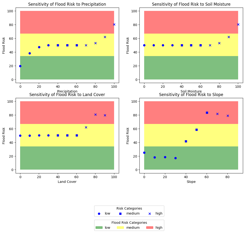
To interpret the plot, observe how the flood risk changes as the input variable value increases or decreases. A steep slope in the plot indicates that the flood risk is highly sensitive to changes in the input variable. If the flood risk remains relatively constant despite changes in the input variable, it suggests that the flood risk is less sensitive to that input variable.
To understand the meaning of the plot, consider that it represents how much the flood risk is affected by each input variable, given that other input variables are kept constant. By analyzing the plot, you can identify which input variables have a more significant impact on flood risk and prioritize interventions or mitigation strategies accordingly.
4 Summary
Flood risk assessment is a critical component of disaster management and urban planning. Accurate and reliable flood risk estimation helps authorities make informed decisions, prioritize resources, and implement effective mitigation strategies. With the increasing impacts of climate change and urbanization, there is a growing need for advanced techniques that can provide better insights into flood risk under varying conditions.
Fuzzy Inference Systems (FIS) offer a robust and flexible approach to model complex relationships between multiple input variables and an output variable, such as flood risk. By incorporating expert knowledge and handling uncertainties, FIS models can capture the intricacies of real-world systems, providing more accurate and reliable estimates of flood risk compared to traditional methods.
FIS models have gained popularity in the field of hydrological modeling and flood risk assessment due to their ability to handle imprecise and incomplete data, as well as their capability to incorporate human reasoning and intuition in the form of linguistic rules. This ability to integrate expert knowledge with quantitative data provides a valuable advantage, especially in situations where data availability is limited or uncertain.
The utilization of FIS in flood risk assessment typically involves defining input variables that influence flood risk, such as precipitation intensity, soil moisture, land cover, and slope. These variables are then used to estimate the flood risk level, which can be categorized into different levels, such as low, medium, or high.
To build an FIS model for flood risk assessment, the first step is to identify relevant input variables and their value domains. Next, fuzzy sets and membership functions are defined for each variable, followed by the formulation of fuzzy rules that describe the relationship between input variables and flood risk. These rules are derived from expert knowledge or empirical data and are used to determine the output flood risk level.
One of the critical aspects of FIS models is their ability to handle uncertainties and vagueness in the input data. This is particularly important in the context of flood risk assessment, where data can be scarce or subject to significant measurement errors. By using fuzzy sets and membership functions, FIS models can accommodate these uncertainties, providing more reliable and robust estimates of flood risk.
Sensitivity analysis is a valuable tool for evaluating the performance of FIS models in flood risk assessment. By varying input variables within their expected range and studying the corresponding changes in flood risk, modelers can gain insight into the behavior of the model and identify any unrealistic responses or potential areas for improvement.
FIS models can be further enhanced by incorporating optimization techniques to identify the most critical factors contributing to flood risk. This can help decision-makers focus on specific areas or interventions that have the most significant impact on reducing flood risk and improving overall resilience.
One of the challenges in applying FIS models for flood risk assessment is the lack of observed data for model validation. In such cases, the performance of the model can be evaluated using expert knowledge, sensitivity analysis, comparison with other models, or the use of simulated data from hydrological or hydraulic models.
In conclusion, FIS provides a promising approach for flood risk assessment, offering a flexible and robust framework for modeling complex relationships and handling uncertainties. By incorporating expert knowledge and quantitative data, FIS models have the potential to significantly improve our understanding of flood risk and support more effective decision-making in disaster management and urban planning.