Correct the parameters, not the data
A resolution mismatch I have been stuck on.
The satellite product I want to correct sits on a 0.1 degree grid. The gauge-based reference I want to correct it towards sits on a 0.5 degree grid. One reference cell covers a 5 by 5 block of satellite pixels: twenty-five of mine inside one of theirs.
The obvious move is to regrid. Interpolate the reference up to 0.1 degree, then correct pixel by pixel against it.
I did that first. It works, in the sense that it runs and produces numbers. It also throws away the thing I most wanted to keep.
What regridding costs
The satellite’s whole value here is spatial detail. It sees the ridge and the valley separately. It knows the rain shadow is dry. That detail is the reason to use a satellite product at all instead of just interpolating gauges, which is what the reference already is.
When you interpolate a 0.5 degree field up to 0.1 degree, you do not create detail. You create twenty-five copies of one number, smoothed a bit at the edges. Then you correct each satellite pixel towards its share of that smoothed field, and the correction drags all twenty-five pixels towards the same target.
The satellite detail is still technically in there, but you have applied a spatially uniform pull across each block. The correction cannot know that one of those pixels is a ridge and another is a valley, because the reference cannot know it either.
The alternative, which is not obvious until it is
Wood and colleagues worked this out in a downscaling context twenty years ago, and it is usually called BCSD. The idea reverses the order of operations.
Do not interpolate the rainfall. Interpolate the correction.
Concretely: fit the distribution parameters on the reference’s own native grid, where the data actually lives and where each value is supported by the stations that went into it. That gives you a coarse, blocky field of parameters, one set per 0.5 degree cell. Then interpolate those parameters down to 0.1 degree, and quantile-map each satellite pixel against its own locally interpolated target distribution.
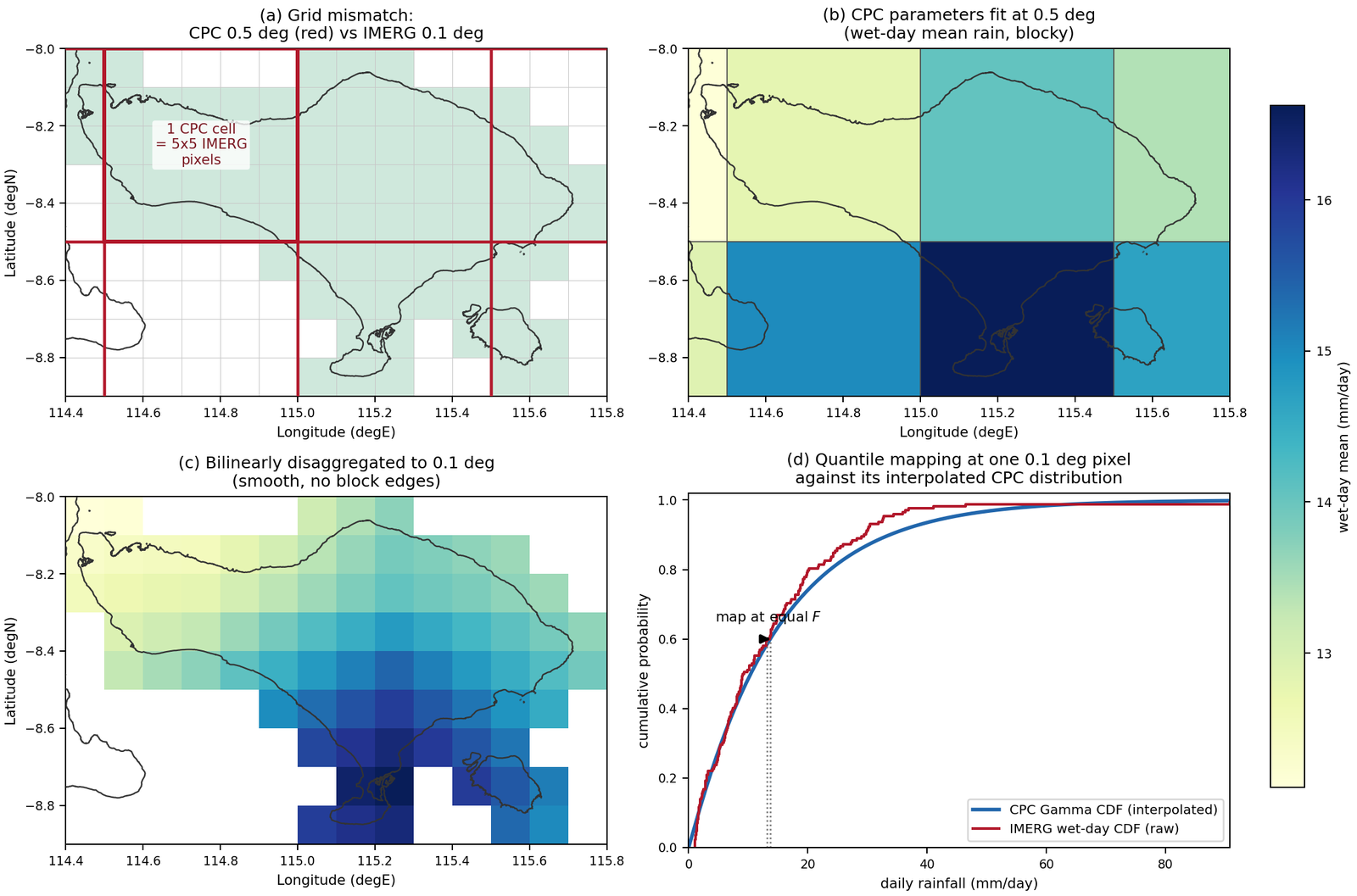
The difference is subtle and it matters. The parameters are climatological. They describe the shape of the rainfall distribution over twenty-odd years, not what fell on any particular day. Climatology varies smoothly in space in a way that daily rainfall emphatically does not. So interpolating a shape parameter across 50 km is a defensible thing to do, where interpolating Tuesday’s rainfall across 50 km is not.
Meanwhile the satellite keeps every bit of its native resolution, because nothing was ever done to the rainfall field itself. Each pixel gets its own target distribution, slightly different from its neighbour’s, and gets mapped against that.
Why it took me a while to see
I think the reason this is not the first thing you reach for is that “make the grids match” feels like a prerequisite rather than a choice. Two datasets, different resolutions, so obviously step one is to put them on the same grid.
But the grids do not actually need to match. Only the parameters do. Once you separate the correction from the data it is correcting, the resolution problem moves from the rainfall, where it is destructive, to the climatology, where it is nearly harmless.
There is a caveat I want to record. The parameters are still only as good as the reference underneath them, and that reference is a gauge interpolation whose quality varies enormously across the country. Making the parameters smooth does not make them right. It makes them smoothly wrong in the places where the reference was weak to begin with, and it does not tell you where those places are.
That problem is not solved by BCSD and I do not have an answer for it yet.
The code
Two functions, and the split between them is the whole idea. The first fits on the coarse grid where the data lives. The second moves the fitted parameters, not the rainfall, down to the fine grid.
def fit_cpc_parameters_on_native_grid(
        cpc_native_dekad
    ):
    """
    Fit gamma and GPD distribution parameters at each CPC native-resolution cell.

    This avoids redundantly fitting the same CPC time series 25 times (as happens
    when CPC is nearest-neighbour regridded to 0.1°). Instead, parameters are
    fitted once per ~0.5° cell and later interpolated to the IMERG grid.

    Based on the BCSD principle (Wood et al. 2004): correct at reference resolution,
    then disaggregate smoothly.

    Parameters
    ----------
    cpc_native_dekad : xarray.DataArray
        CPC precipitation at native ~0.5° resolution for one dekad across all years.
        Shape (n_time, n_lat_cpc, n_lon_cpc).

    Returns
    -------
    dict of xarray.DataArray
        Dictionary with 9 parameter arrays at CPC native resolution:
        'gamma_shape', 'gamma_scale', 'gpd_threshold', 'gpd_shape',
        'gpd_loc', 'gpd_scale', 'upper_cap', 'p_threshold', 'p_dry_cpc'.
        Ocean/invalid cells are NaN.

    Notes
    -----
    Fixes applied (2026.04):
      * Fix C (Cannon 2015 §3.2): gamma distribution fitted on WET-day values
        only (> WET_DAY_THRESHOLD), not on all values including zeros. The
        GPD threshold is also computed from wet values only.
      * Fix A (Coles 2001): GPD fitting inside cross_validate_gpd uses
        floc=0 (see fit_generalized_pareto_distribution).
      * New: p_dry_cpc is returned per cell so the downstream mapping
        step can apply Cannon dry-day handling using the interpolated
        dry-day frequency at each IMERG pixel.
    """
    lat_cpc = cpc_native_dekad.lat.values
    lon_cpc = cpc_native_dekad.lon.values
    n_lat = len(lat_cpc)
    n_lon = len(lon_cpc)

    # Initialize parameter arrays with NaN
    param_names = [
        'gamma_shape', 'gamma_scale', 'gpd_threshold',
        'gpd_shape', 'gpd_loc', 'gpd_scale',
        'upper_cap', 'p_threshold', 'p_dry_cpc'
    ]
    params = {
        name: np.full((n_lat, n_lon), np.nan)
        for name in param_names
    }

    import time as _time
    _fitted = 0
    _skipped = 0
    _t0 = _time.time()

    for i in range(n_lat):
        for j in range(n_lon):
            ts = cpc_native_dekad.values[:, i, j]

            # Skip all-NaN cells (ocean)
            if np.all(np.isnan(ts)):
                _skipped += 1
                continue

            # Remove NaN and split into wet-day sample (Fix C, Cannon 2015)
            valid = ts[~np.isnan(ts)]
            wet = valid[valid > WET_DAY_THRESHOLD]

            # Need sufficient wet-day data for fitting
            if len(wet) < 10:
                _skipped += 1
                continue

            # Dry-day fraction (new: required by downstream Cannon mapping)
            params['p_dry_cpc'][i, j] = 1.0 - (len(wet) / len(valid))

            # Fit gamma on wet-day sample only
            shape, _loc, scale = fit_gamma_distribution(wet)
            if shape <= 0 or scale <= 0:
                _skipped += 1
                continue

            params['gamma_shape'][i, j] = shape
            params['gamma_scale'][i, j] = scale

            # GPD threshold (80th percentile of WET values, Fix C)
            threshold = np.percentile(wet, GPD_THRESHOLD_PERCENTILE)
            params['gpd_threshold'][i, j] = threshold

            # Fit GPD via cross-validation on the wet sample (Fix A inside)
            if not np.isnan(threshold) and threshold > 0:
                gpd_shape, gpd_loc, gpd_scale = cross_validate_gpd(wet, threshold)
                params['gpd_shape'][i, j] = gpd_shape
                params['gpd_loc'][i, j] = gpd_loc
                params['gpd_scale'][i, j] = gpd_scale
            else:
                params['gpd_shape'][i, j] = 0
                params['gpd_loc'][i, j] = 0
                params['gpd_scale'][i, j] = 1

            # Upper cap (99.9th percentile of wet values)
            params['upper_cap'][i, j] = np.percentile(wet, UPPER_CAP_THRESHOLD_PERCENTILE)

            # Pre-compute CDF at threshold for conditional probability mapping
            params['p_threshold'][i, j] = gamma.cdf(threshold, shape, loc=0, scale=scale)

            _fitted += 1

        # Progress every 5 rows
        if (i + 1) % 5 == 0 or (i + 1) == n_lat:
            elapsed = _time.time() - _t0
            pct = (i + 1) / n_lat * 100
            eta = elapsed / (i + 1) * (n_lat - i - 1) if i > 0 else 0
            logging.info(
                f"  Native CPC fitting: row {i+1}/{n_lat} ({pct:.0f}%) "
                f"| {_fitted} fitted, {_skipped} skipped "
                f"| elapsed {elapsed:.0f}s, ETA {eta:.0f}s"
            )

    logging.info(f"Fitted CPC params on native grid: {_fitted}/{n_lat * n_lon} cells")

    # Convert to xarray DataArrays
    cpc_params = {}
    for name in param_names:
        cpc_params[name] = xr.DataArray(
            params[name],
            coords={'lat': lat_cpc, 'lon': lon_cpc},
            dims=['lat', 'lon'],
            name=name
        )

return cpc_paramsdef interpolate_cpc_params_to_imerg_grid(
cpc_params,
target_lat,
target_lon
):
"""
Bilinearly interpolate CPC distribution parameters from native ~0.5° to
the IMERG 0.1° grid. Uses a two-pass approach: bilinear first, then
nearest-neighbour to fill boundary NaN values.
Parameters
----------
cpc_params : dict of xarray.DataArray
CPC distribution parameters at native resolution, as returned by
fit_cpc_parameters_on_native_grid().
target_lat : numpy.ndarray
Target latitude values (IMERG grid).
target_lon : numpy.ndarray
Target longitude values (IMERG grid).
Returns
-------
dict of xarray.DataArray
Interpolated parameters at IMERG resolution.
"""
interp_params = {}
for name, param_da in cpc_params.items():
# Pass 1: bilinear interpolation (NaN outside the convex hull of
# CPC-native cell centres; bites small AOIs where the AOI extent
# reaches outside the centres, e.g. Bali on a 2 x 4 CPC tile).
interp_da = param_da.interp(
lat=target_lat, lon=target_lon, method='linear'
)
# Pass 2: fill boundary NaN with true unrestricted nearest-neighbour.
# Note: interp(method='nearest') ALSO returns NaN beyond the convex
# hull (it goes through scipy.interpolate with bounds_error=False),
# which silently broke small AOIs. reindex(method='nearest') is a
# pure lookup with no convex-hull restriction.
n_nan_before = int(interp_da.isnull().sum().item())
if n_nan_before > 0:
nearest_da = param_da.reindex(
lat=target_lat, lon=target_lon, method='nearest'
)
interp_da = interp_da.fillna(nearest_da)
interp_params[name] = interp_da
# Validate: clip gamma shape/scale to small positive minimum
for key in ('gamma_shape', 'gamma_scale'):
if key in interp_params:
interp_params[key] = interp_params[key].clip(min=1e-6)
# Clip p_dry_cpc to [0, 1] - bilinear interpolation of a probability
# can numerically drift slightly outside the valid range.
if 'p_dry_cpc' in interp_params:
interp_params['p_dry_cpc'] = interp_params['p_dry_cpc'].clip(min=0.0, max=1.0)
# Log summary
sample_key = 'gamma_shape'
n_valid = int((~interp_params[sample_key].isnull()).sum().item())
n_total = int(np.prod(interp_params[sample_key].shape))
logging.info(
f"Interpolated CPC params to IMERG grid: "
f"{n_valid}/{n_total} valid pixels"
)
return interp_params