Calculate SPI using monthly rainfall data in GeoTIFF format

NOTES - 1 Mar 2022

I have write a new and comprehensive guideline on SPI, you can access via this link https://bennyistanto.github.io/spi/

---

These last few months, I have tried a lot of difference formulation to calculate Standardized Precipitation Index (SPI) based on rainfall data in netCDF format, check below blog post as a background:

1. SPI using IMERG

2. SPI using CHIRPS

The reason why I use rainfall in netCDF format in above blog post because the software to calculate SPI: climate-indices python package will only accept single netCDF as input, and the SPI script will read the netCDF input file based on time dimension.

Converting raster files into netCDF is easy using GDAL or other GIS software, but to make the time dimension enabled netCDF output and CF-Compliant is another story. Using NCO, I can easily rename any variable with ncrename and add attributes to the content with ncatted to fit the desired data structure. Yet, I think this is too much work if every time I update the data, I should update the attribute too.

Then I found this solution.

Now, I am able to convert bunch of GeoTIFF in a folder into a single netCDF file with time dimension enabled and CF-Compliant and can be accepted as input using climate-indices software.

Lets try!

This step-by-step guide was tested using Macbook Pro, 2.9 GHz 6-Core Intel Core i9, 32 GB 2400 MHz DDR4, running on macOS Big Sur 11.1

0. Working directory

For this test, I am working at /Users/bennyistanto/Temp/CHIRPS/SPI/Java directory. I have some folder inside this directory:

1. Download

2. Fitting

3. Input_nc

4. Input_TIF

5. Output_nc

6. Output_TEMP

7. Output_TIF

8. Script

9. Subset

Feel free to use your own preferences for this setting.

1. Software requirement

The installation and configuration described below are performed using a bash/zsh shell on macOS. Windows users will need to install and configure a bash shell in order to follow the instruction below. Try to use Windows Subsystem for Linux for this purpose.

1.1. If you are new to using Bash refer to the following lessons with Software Carpentry: http://swcarpentry.github.io/shell-novice/

1.2. If you don't have Homebrew, you can install it by pasting below code in your macOS terminal.

• bin/bash -c "$(curl -fsSL https://raw.githubusercontent.com/Homebrew/install/master/install.sh)"

1.3. Install wget (for downloading data). Use Hombrew to install it by pasting below code in your macOS terminal.

• brew install wget

1.4. Download and install Panoply Data Viewer from NASA GISS on your machine: macOS, Windows, Linux.

1.5. Download and install Anaconda Python on your machine: macOS, Windows, Linux.

1.6. Or you can use Miniconda: macOS, Windows, Linux

2. Configure the python environment

The code for calculating SPI is written in Python 3. It is recommended to use either the Miniconda3 (minimal Anaconda) or Anaconda3 distribution. The below instructions will be Anaconda specific (although relevant to any Python virtual environment), and assume the use of a bash shell.

A new Anaconda environment can be created using the conda environment management system that comes packaged with Anaconda. In the following examples, I’ll use an environment named climate_indices (any environment name can be used instead of climate_indices) which will be created and populated with all required dependencies through the use of the provided setup.py file.

2.1. First, create the Python environment:

• conda create -n climate_indices python=3.7

2.2. The environment created can now be ‘activated’:

• conda activate climate_indices

2.3. Install climate-indices package. Once the environment has been activated then subsequent Python commands will run in this environment where the package dependencies for this project are present. Now the package can be added to the environment along with all required modules (dependencies) via pip:

• pip install climate-indices

2.4. Install Climate Data Operator (CDO) from Max-Planck-Institut für Meteorologie using conda

• conda install -c conda-forge cdo

2.5. Install netCDF Operator (NCO) using conda

• conda install -c conda-forge nco

2.6. Install jupyter and other package using conda

• conda install -c conda-forge jupyter numpy datetime gdal netCDF4

3. Rainfall data acquisition

SPI requires monthly rainfall data, and there are many source providing global high-resolution gridded monthly rainfall data:

• CHIRPS

• IMERG

• FLDAS

• TerraClimate

• CRU

For this step-by-step guideline, I will use CHIRPS monthly data in GeoTIFF format and the case study is Java island - Indonesia.

Why CHIRPS? It is produced at 0.05 x 0.05 degree spatial resolution, make it CHIRPS is the highest gridded rainfall data, and long-term historical data from 1981 – now.

3.1. Navigate to Download folder in the working directory. Download using wget all CHIRPS monthly data in GeoTIFF format from Jan 1981 to Dec 2020 (this is lot of data ~7GB zipped files, and become 27GB after extraction, please make sure you have bandwidth and unlimited data package):

• wget -r https://data.chc.ucsb.edu/products/CHIRPS-2.0/global_monthly/tifs/

3.2. Gunzip all the downloaded files

• gunzip *.gz

3.3. Download the Java boundary shapefile http://on.istan.to/365PSyH. And save it in Subset directory then unzip it.

3.4. Still in your Download directory, Clip your area of interest using Java boundary and save it to Input_TIF directory. I will use gdalwarp command from GDAL to clip all GeoTIFF files in a folder.

• for i in `find *.tif`; do gdalwarp --config GDALWARP_IGNORE_BAD_CUTLINE YES -srcnodata NoData -dstnodata -9999 -cutline ../Subset/java_bnd_chirps_subset.shp $i ../Input_TIF/java_cli_$i; done

  if you are using Windows, you can follow below script.

• for %i IN (*.tif) do gdalwarp --config GDALWARP_IGNORE_BAD_CUTLINE YES -srcnodata NoData -dstnodata -9999 -cutline ../Subset/java_bnd_chirps_subset.shp %i ../Input_TIF/java_%i

  If you have limited data connection or lazy to download ~7GB and process ~27GB data, you can get pre-processed clipped data for Java covering Jan 1981 to Dec 2020, with file size ~6.8MB. Link: https://on.istan.to/3iLu68v

3.4. Download python script/notebook that I use to convert GeoTIFF in a folder to single netCDF, save it to Script folder.

• Python script: https://gist.github.com/bennyistanto/ff16dc08cc06b5a13740323db41dc8f3 or https://s3.benny.istan.to/script/tiff2nc.py

• Jupyter notebook: https://github.com/wfpidn/VAMscript/blob/master/notebook/CHIRPS-GeoTIFF_to_netCDF_Java.ipynb or https://s3.benny.istan.to/script/CHIRPS-GeoTIFF_to_netCDF_Java.ipynb

You MUST adjust the folder location (replace /path/to/directory/ with yours) in line 13 and 114.

If you are using other data source (I assume all the data in WGS84), you need to adjust few code in:

• Line 31: folder location

• Line 40: start of the date

• Line 44: output name

• Line 53: date attribute

• Line 85-88: bounding box

• Line 110: output filename structure

• Line 114: folder location

• Line 120-122: date character location in a filename

3.5. After everything is set, then you can execute the translation process

• Using Python in Terminal, navigate to your Script directory, type python tiff2nc.py

• Wait for a few moments, you will get the output java_cli_chirps_1months_1981_2020.nc. You will find this file inside Input_TIF folder. Move it to Input_nc folder.

• Using Jupyter, make sure you still inside conda climate_indices environment, type in Terminal jupyter notebook

• Navigate to your notebook directory (where you put *.ipynb file), run Cell by Cell until completed. Wait for a few moments, you will get the output java_cli_chirps_1months_1981_2020.nc. You will find this file inside Input_TIF folder. Move it to Input_nc folder.

• You also can get this data: java_cli_chirps_1months_1981_2020.nc via this link http://on.istan.to/3iRDl7e

4. Calculate SPI

The climate-indices software enables the user to calculate SPI using any gridded netCDF dataset, However, there are certain specifications for input files that vary based on input type.

• Precipitation unit must be written as 'millimeters', 'milimeter', 'mm', 'inches', 'inch' or 'in'

• Data dimension and order must be written as 'lat', 'lon', 'time' or 'time', 'lat', 'lon'

4.1. I have try to make script in Step 3.4. are follow above specification. To make sure everything is correct, in your Terminal - navigate to your directory where you save java_cli_chirps_1months_1981_2020.nc file: Input_nc. Then type ncdump -h java_cli_chirps_1months_1981_2020.nc

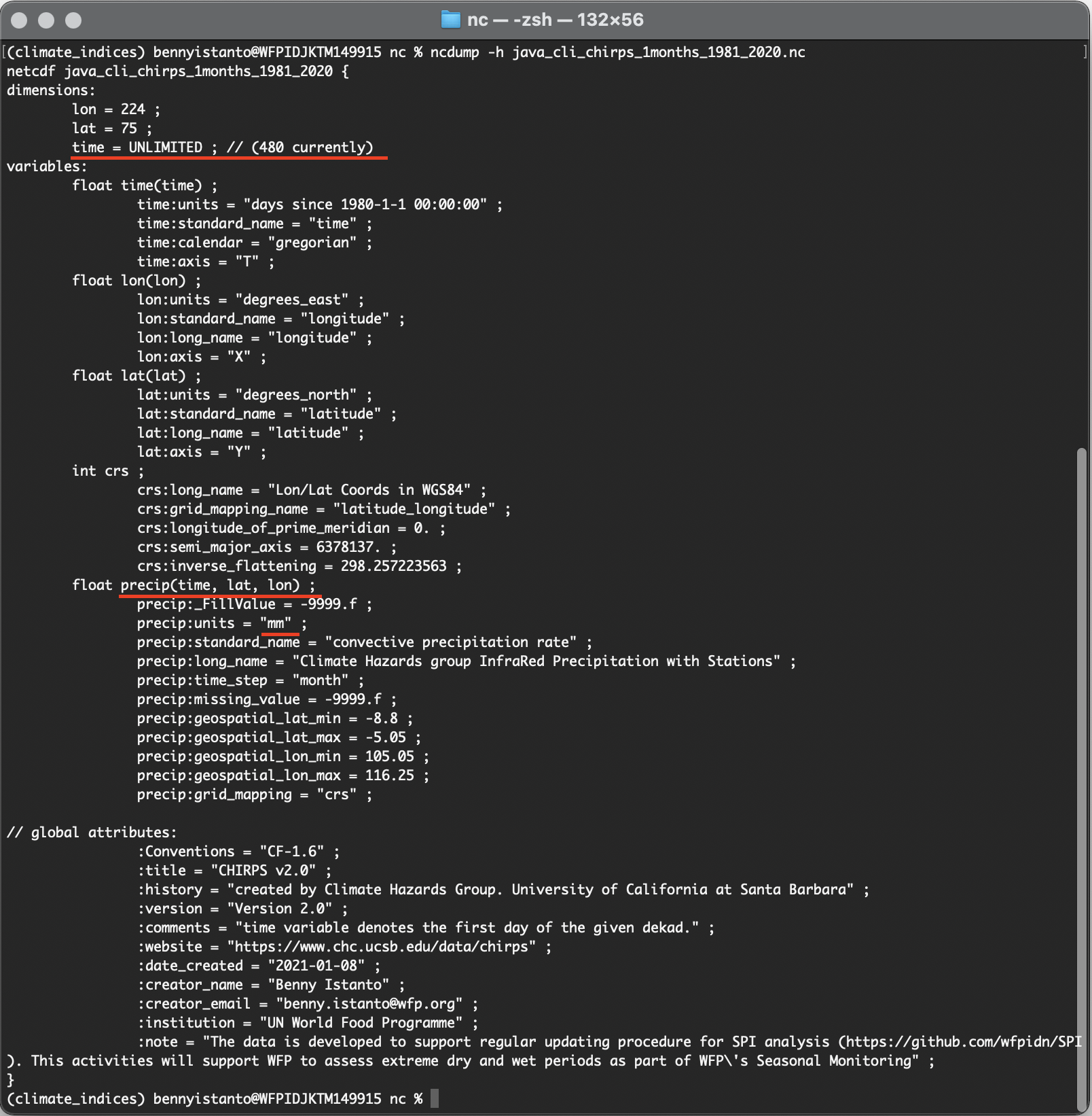
From above picture, I can say:

• Time dimension is enabled, 480 is total months from Jan 1981 to Dec 2020

• Data dimension and order are following the specification 'time', 'lat', 'lon'

• The unit is in 'mm'

So, everything is correct and I am ready to calculate SPI. Make sure in your Terminal still inside climate_indices environment.

Other requirements and options related to the indices calculation, please follow https://climate-indices.readthedocs.io/en/latest/#indices-processing

4.2. In order to pre-compute fitting parameters for later use as inputs to subsequent SPI calculations I can save both gamma and Pearson distribution fitting parameters to NetCDF, and later use this file as input for SPI calculations over the same calibration period.

In your Terminal, run the following code.

$ spi --periodicity monthly --scales 1 2 3 6 9 12 24 36 48 60 72 --calibration_start_year 1981 --calibration_end_year 2020 --netcdf_precip /Users/bennyistanto/Temp/CHIRPS/Java/Input_nc/java_cli_chirps_1months_1981_2021.nc --var_name_precip precip --output_file_base /Users/bennyistanto/Temp/CHIRPS/Java/Output_nc/java_CHIRPS --multiprocessing all --save_params /Users/bennyistanto/Temp/CHIRPS/Java/Fitting/java_CHIRPS_fitting.nc --overwrite

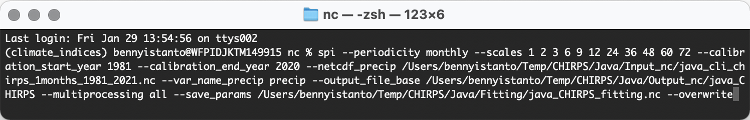
The above command will compute SPI (standardized precipitation index, both gamma and Pearson Type III distributions) from an input precipitation dataset (in this case, CHIRPS precipitation dataset). The input dataset is monthly rainfall accumulation data and the calibration period used will be Jan-1981 through Dec-2020. The index will be computed at 1,2,3,6,9,12,24,36,48,60 and 72-month timescales. The output files will be <out_dir>/java_CHIRPS_spi_gamma_xx.nc, and <out_dir>/java_CHIRPS_spi_pearson_xx.nc.

The output files will be:

• 1-month: /Output_nc/java_CHIRPS_spi_gamma_01.nc

• 2-month: /Output_nc/java_CHIRPS_spi_gamma_02.nc

• 3-month: /Output_nc/java_CHIRPS_spi_gamma_03.nc

• 6-month: /Output_nc/java_CHIRPS_spi_gamma_06.nc

• 9-month: /Output_nc/java_CHIRPS_spi_gamma_09.nc

• 12-month: /Output_nc/java_CHIRPS_spi_gamma_12.nc

• 24-month: /Output_nc/java_CHIRPS_spi_gamma_24.nc

• 36-month: /Output_nc/java_CHIRPS_spi_gamma_36.nc

• 48-month: /Output_nc/java_CHIRPS_spi_gamma_48.nc

• 60-month: /Output_nc/java_CHIRPS_spi_gamma_60.nc

• 72-month: /Output_nc/java_CHIRPS_spi_gamma_72.nc

• 1-month: /Output_nc/java_CHIRPS_spi_pearson_01.nc

• 2-month: /Output_nc/java_CHIRPS_spi_pearson_02.nc

• 3-month: /Output_nc/java_CHIRPS_spi_pearson_03.nc

• 6-month: /Output_nc/java_CHIRPS_spi_pearson_06.nc

• 9-month: /Output_nc/java_CHIRPS_spi_pearson_09.nc

• 12-month: /Output_nc/java_CHIRPS_spi_pearson_12.nc

• 24-month: /Output_nc/java_CHIRPS_spi_pearson_24.nc

• 36-month: /Output_nc/java_CHIRPS_spi_pearson_36.nc

• 48-month: /Output_nc/java_CHIRPS_spi_pearson_48.nc

• 60-month: /Output_nc/java_CHIRPS_spi_pearson_60.nc

• 72-month: /Output_nc/java_CHIRPS_spi_pearson_72.nc

Parallelization will occur utilizing all CPUs.

For small area of interest, the calculation will fast and don’t take much time. Below is example if you processed bigger area:

• Monthly IMERG data, global coverage 180W - 180E, 60N - 60S, 0.1 deg spatial resolution. It takes almost 9-hours to process SPI 1-72 months.

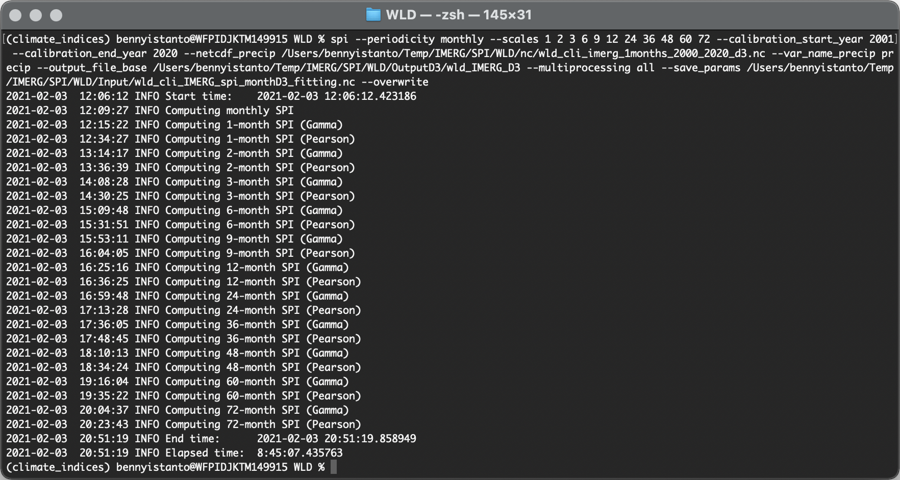
Output gamma and pearson file https://on.istan.to/2MhVnTP

Fitting file http://on.istan.to/3c6ZLjq

5. Updating procedure when new data is available

What if the new data is coming (Jan 2021)? Should I re-run again for the whole periods, 1981 to date? That's not practical as it requires large storage and time processing if you do for bigger coverage (country or regional analysis).

Updating SPI up to SPI72, I should have data at least 6 years back (2014) from the latest (Jan 2021). In order to avoid computation for the whole periods (1981-2021), I will process data data only for year 2014 to 2021.

After that, I continue the process following Step 3.4.

Step 4.2 demonstrates how distribution fitting parameters can be saved as NetCDF. This fittings NetCDF can then be used as pre-computed variables in subsequent SPI computations. Initial command computes both distribution fitting values and SPI for various month scales.

The distribution fitting variables are written to the file specified by the ’--save_params’ option.

The second command also computes SPI but instead of computing the distribution fitting values it loads the pre-computed fitting values from the NetCDF file specified by the ’--load_params’ option.

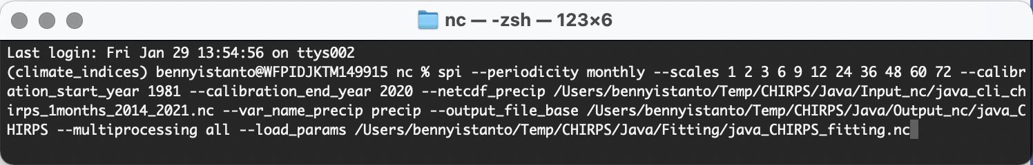
See below code:

$ spi --periodicity monthly --scales 1 2 3 6 9 12 24 36 48 60 72 --calibration_start_year 1981 --calibration_end_year 2020 --netcdf_precip /Users/bennyistanto/Temp/CHIRPS/Java/Input_nc/java_cli_chirps_1months_2014_2021.nc --var_name_precip precip --output_file_base /Users/bennyistanto/Temp/CHIRPS/Java/Output_nc/java_CHIRPS --multiprocessing all --load_params /Users/bennyistanto/Temp/CHIRPS/Java/Fitting/java_CHIRPS_fitting.nc

6. Visualized the result using Panoply

Let see the result.

6.1. From the Output_nc directory, right-click file java_CHIRPS_spi_gamma_3_month.nc (you can download this file from this link: https://on.istan.to/2MhVnTP) and Open With Panoply.

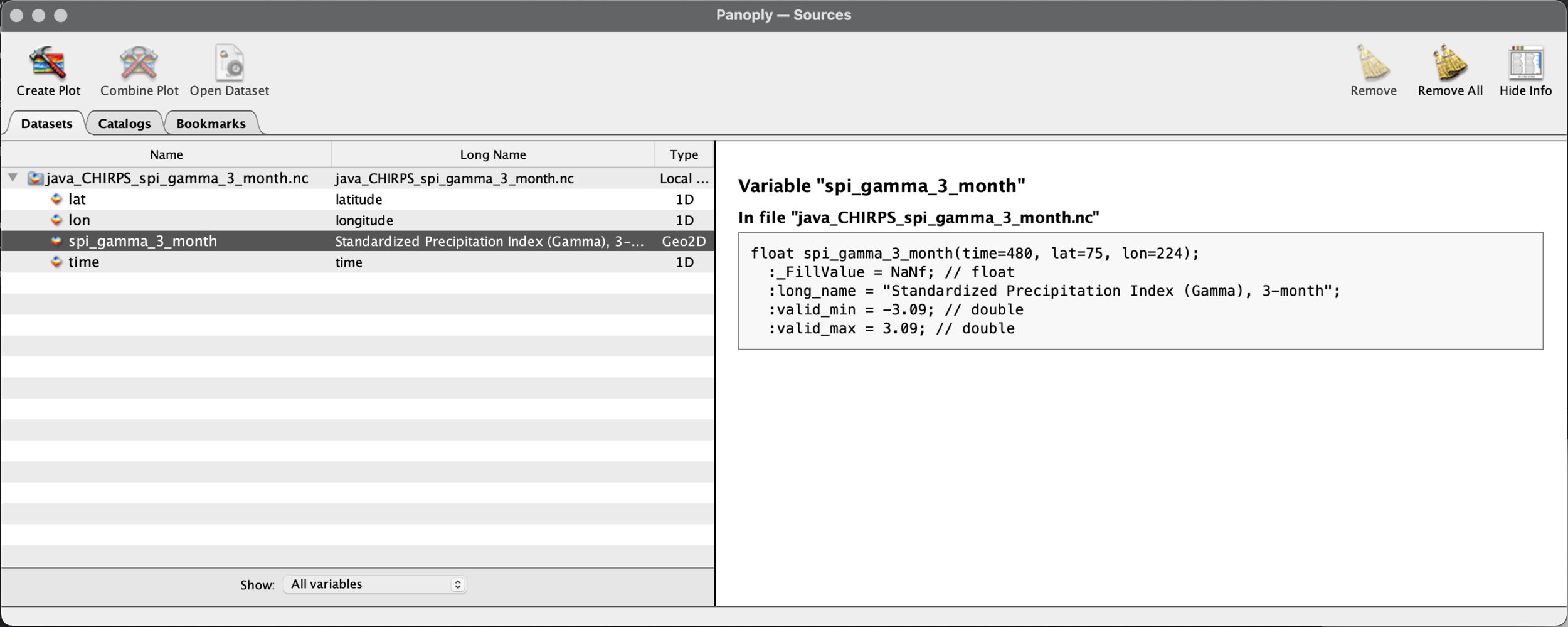
6.2. From the Datasets tab select spi_gamma_3_month and click Create Plot

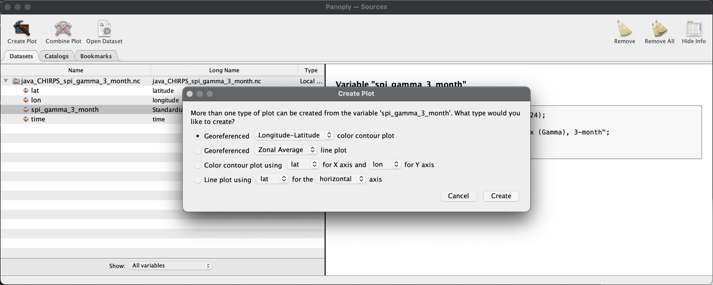
6.3. In the Create Plot window select option Georeferenced Longitude-Latitude.

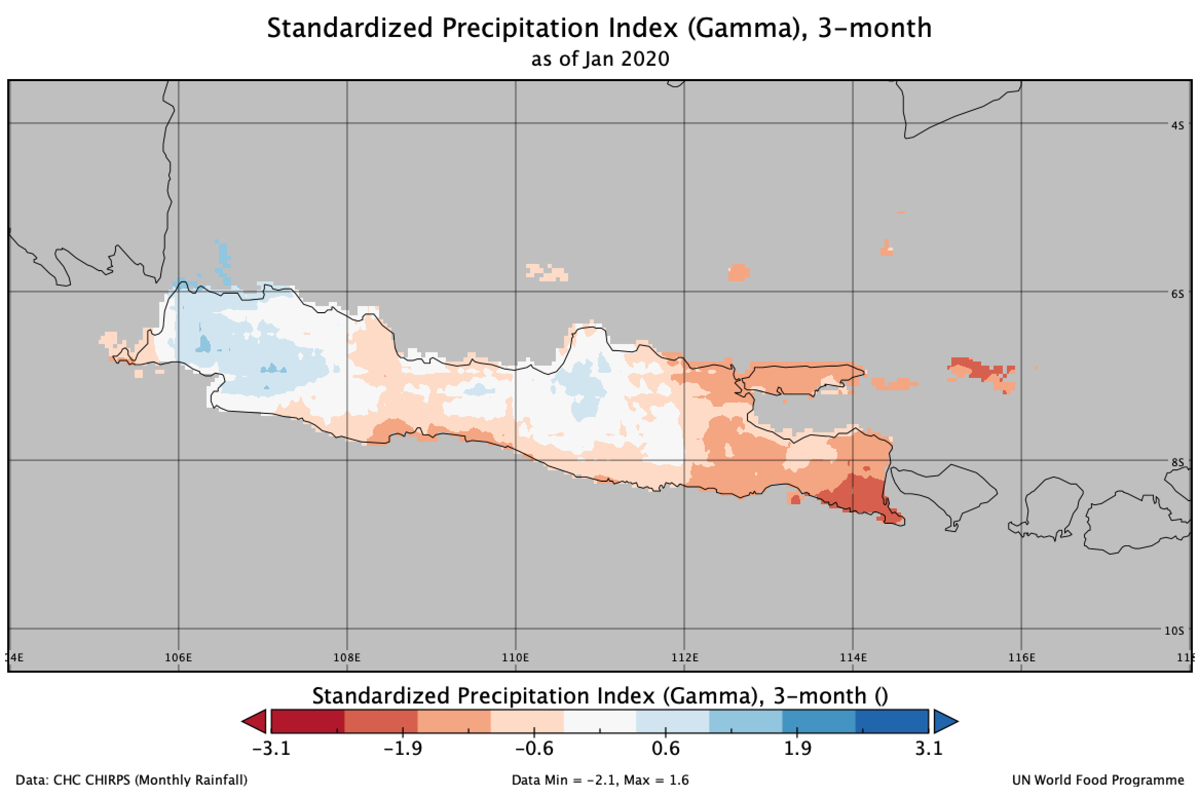
6.4. When the Plot window opens:

• Array tab: Change the time into 469 to view data on Jan 2020

• Scale tab: Change value on Min -3, Max 3, Major 6, Color Table CB_RdBu_09.cpt

• Map tab: Change value on Center on Lon 110.0 Lat -7.5, then Zoom in the map through menu-editor Plot > Zoom Plot In few times until Indonesia appear proportionally. Set grid spacing 2.0 and Labels on every grid lines.

• Overlays tab: Change Overlay 1 to MWDB_Coasts_Countries_1.cnob

7. Convert the result to GeoTIFF

Conversion of the result into GeoTIFF format, CDO required the variable should be in "time, lat, lon", while the output from SPI: java_CHIRPS_spi_xxxxx_x_month.nc in "lat, lon, time", you can check this via ncdump -h file.nc

• Navigate your Terminal to folder Output_nc

• Let's re-order the variables into time,lat,lon using ncpdq command from NCO and save the result to folder Output_TEMP

  • ncpdq -a time,lat,lon java_CHIRPS_spi_gamma_3_month.nc ../Output_TEMP/java_CHIRPS_spi_gamma_3_month_rev.nc

• Navigate your Terminal to folder Output_TEMP

• Check result and metadata to make sure everything is correct.

  • ncdump -h java_CHIRPS_spi_gamma_3_month_rev.nc

• Then convert all SPI value into GeoTIFF with time dimension information as the filename using CDO and GDAL.

• Navigate your Terminal to folder Output_TEMP and save the result to folder Output_TIF

  • for t in `cdo showdate java_CHIRPS_spi_gamma_3_month_rev.nc`; do

    cdo seldate,$t java_CHIRPS_spi_gamma_3_month_rev.nc dummy.nc

    gdal_translate -of GTiff -a_ullr 105.05 -5.05 116.25 -8.8 -a_srs EPSG:4326 -co COMPRESS=LZW -co PREDICTOR=1 dummy.nc ../Output_TIF/$t.tif

    done

FINISH

Congrats, now you are able to calculate SPI based on monthly rainfall in GeoTIFF format.