Second-order Markov chain model to generate time series of occurrence and rainfall
1 Introduction
In the realm of meteorological studies, the use of statistical models is pivotal for understanding and predicting various weather phenomena. Among these models, the second-order Markov chain model has emerged as a powerful tool, particularly in generating time series of rainfall occurrence (Wilks, 1998). This model provides a robust framework for simulating rainfall patterns, offering valuable insights that are crucial for weather forecasting, water resource management, and climate change studies.
The second-order Markov chain model distinguishes itself from its first-order counterpart through its ability to consider not just the state of the system at the previous time step, but also the state at the time step before that. This additional layer of historical context allows the model to capture more complex dependencies and transitions in the rainfall data (Bellone et al., 2000). This enhanced capability significantly improves the accuracy of the generated time series, making it a powerful tool in the study of rainfall patterns.
Rainfall, as a natural phenomenon, exhibits a high degree of variability and randomness. The second-order Markov chain model, with its ability to incorporate historical context, is well-equipped to handle this variability (Hughes et al., 1999). By considering the state of the system at two previous time steps, the model can capture the inherent randomness in rainfall occurrence, thereby generating a time series that closely mirrors real-world rainfall patterns.
The application of the second-order Markov chain model to rainfall data is not just a theoretical exercise. The generated time series of rainfall occurrence can have practical applications in various fields. For instance, in the field of agriculture, understanding rainfall patterns can help farmers plan their planting and harvesting schedules (Rosenzweig et al., 2000). In urban planning, accurate rainfall predictions can inform the design of drainage systems to prevent flooding (Ashley et al., 2005).
2 Data
Over the past three decades, Bogor’s climate has remained relatively consistent. The city experiences an average annual temperature of around 26 °Celsius. The temperature varies little throughout the year, with the warmest month averaging around 27 °Celsius and the coolest month averaging around 25 °Celsius.
In terms of rainfall, Bogor receives an average annual precipitation of over 3,000 millimeters. The city experiences the most rainfall from November to March, with each of these months receiving over 300 millimeters of rain on average. Even in the driest months, from June to September, Bogor still receives over 100 millimeters of rain per month on average.
This consistent and significant rainfall, combined with the city’s warm temperatures, contributes to its lush, tropical environment. The climatic conditions of Bogor provide a rich dataset for the application of a second-order Markov chain model to generate time series of occurrence and rainfall.
Daily rainfall data of Bogor Climatological Station from 1984-2021 were used in this analysis, downloaded from BMKG Data Online in *.xlsx format. The file then manipulated by remove the logo and unnecessary text, leaving only two columns, namely date in column A and rainfall in column B for the header with the format extending downwards, and save as *.csv format.
The final input file is accessible via this link: https://drive.google.com/file/d/1molqggv9o71Z0VT50h5OvEqCxYq4Bp1Z/view?usp=sharing
3 Methods
This exercise focuses on the second-order Markov chain model as a tool for generating rainfall occurrence probabilities and the gamma distribution for determining rainfall height (Boer, 1999).
The second-order Markov chain model is widely used to represent rainfall occurrence (Stern and Coe, 1984; Hann et al, 1976). In this model, rainfall occurrence on day “i” is influenced by the presence or absence of rainfall in the previous days and the day after the previous day. If rainfall on day “i” is only influenced by rainfall on the previous day, it is considered a first-order Markov chain, and if it is influenced by rainfall two days prior, it is considered a second-order Markov chain, and so on.
The second-order Markov chain model has been demonstrated to be effective in generating time series of rainfall occurrence (Nick and Harp, 1980; Richardson, 1981; Wilks, 1990). Furthermore, the gamma distribution is frequently utilized to determine rainfall height (Wilks, 1990). By employing both the second-order Markov chain model and gamma distribution, this study offers a comprehensive approach to generating rainfall data.
The combined use of the second-order Markov chain model for rainfall occurrence and gamma distribution for rainfall height provides a robust method for generating rainfall data. This approach has significant implications for various fields, such as agriculture and urban planning, where accurate rainfall data is crucial for informed decision-making.
In this exercise, the focus is limited to second-order Markov chains, as the analysis for lower/higher-order chains is fundamentally similar. The analysis employs the symbol 0 for non-rainy days and 1 for rainy days. The probability of rainfall on day i, given that it did not rain on the previous day and the day before previous day, is denoted as P001(i), while the probability of rain given that it rained the previous day and the day before previous day is represented as P111(i). The general form of the estimated probability of rainfall occurrence is as follows:
\[P_{jkl}(i) = \frac{n_{jkl}(i)}{n_{jk0}(i) + n_{jk1}(i)} \tag{1}\]
where njkl(i) represents the number of years in which the event l (0 or 1) occurred on day i, and the event jk (0 or 1) happened on the previous day and the day before the previous day.
3.1 Rainfall occurrence model
Rainfall occurrence models commonly use Fourier regression equations to predict the probability of rainfall occurrence. However, these equations can sometimes produce a fitting line with values greater than 1 or smaller than 0. To address this issue, the probability values are first transformed into a logit function gjkl(i).
\[g_{jkl}(i) = \ln\left(\frac{P_{jkl}(i)}{1 - P_{jkl}(i)}\right) \tag{2}\]
To transform gjkl(i) back into probability values, the following equation is used:
\[P_{jkl}(i) = \frac{1}{1 + \exp(-g_{jkl}(i))} \tag{3}\]
The fitting line for gjkl(i) follows the form presented by Stern and Coe (1984):
\[g_{jkl}(i) = a_0 + a_1 \sin(t'(i)) + b_1 \cos(t'(i)) + a_2 \sin(2t'(i)) + b_2 \cos(2t'(i)) \tag{4}\]
Where \(t'(i) = \frac{2\pi i}{365}\) and \(i = 1, 2, \ldots, 365\)
The number of harmonics, m, can be determined using multiple regression techniques, where independent variables are introduced sequentially, starting with harmonic 1, harmonic 2, and so on until no more variance is explained by the newly introduced variable.
3.2 Rainfall generation model
To generate rainfall data, the probability information required is the probability of rainfall occurrence on day i, where the previous day’s occurrence is k (0 or 1), and the day before yesterday is j (0 or 1). The estimated value for gjkl(i) can be calculated if daily rainfall observation data is available.
For simulation purposes, probability data must be converted into occurrence data. This is done by generating random numbers from a uniform distribution U(0, 1; VanTassel et al., 1990). If the random value from the uniform distribution is smaller than the probability value, it indicates rainfall; otherwise, it indicates no rainfall. If the simulation result indicates rainfall, the next step is to generate rainfall height using theoretical distributions.
The next step in creating a rainfall data simulation model is to calculate the parameters of a theoretical distribution that approximates the rainfall data distribution. The Gamma distribution is widely used to describe rainfall intensity variability (Ison et al., 1971; Stern and Coe, 1984; Waggoner, 1989; Wilks, 1990). The probability density function is as follows:
\[f(x, \alpha, \beta) = \frac{1}{\beta\Gamma(\alpha)}\left(\frac{x}{\beta}\right)^{\alpha-1}e^{-x/\beta} \tag{5}\]
with \(\beta\) being the shape parameter and \(\alpha\) being the scale parameter of the gamma function \(\Gamma\).
Several methods can be employed to estimate the values of the two parameters of the gamma distribution, one of which is the Maximum Likelihood Method. According to Shenton and Bowman (1970, as cited in Haan, 1979), the \(\alpha\) value obtained from the Maximum Likelihood Method may still have a bias, and therefore needs to be corrected. The corrected \(\alpha\) value, calculated using the Greenwood and Durand method, is:
\[FC_\alpha = \frac{(n - 3)\alpha}{n} \tag{6}\]
Subsequently, the \(\beta\) parameter is calculated as follows:
\[\beta = \frac{\bar{X}}{\alpha} \tag{7}\]
The predicted rainfall is based on a predetermined set of patterns, P001, P010, P011 and P111, referred to as P-types. These P-types represent different combinations of previous and future rainy days and are used as event triggers in the model. The rainfall data is then separated into different seasons, DJF, MAM, JJA and SON, based on the month of occurrence. The model takes into account the day-to-day variability within each season.
The gamma distribution, parameterized by \(\alpha\) (shape) and \(\beta\) (scale), is used to generate the predicted rainfall. \(\alpha\) and \(\beta\) parameters for each season are pre calculated. These parameters are fetched for each P-type and season combination.
The random gamma function, employed to simulate rainfall events, generates samples from a Gamma distribution. The number of samples drawn (pertaining to the size parameter in the gamma distribution) ideally aligns with the valid event days within a given season, conforming to the original precipitation data (Wilks, 2011). In essence, for each season and event type, the gamma distribution is simulated as frequently as the number of event days occurring within the season, according to the original data.
Although the simulated events from a uniform distribution and the derived rainfall values from the gamma distribution are not intrinsically connected in the simulation process, they both represent the same event category. To maintain consistency in the temporal distribution of events, the generated rainfall values are matched with the valid event days in the original data. This coherence in the number of samples drawn from the gamma distribution is accomplished by aligning it with the structure of the initial precipitation data, rather than the simulated occurrences. Consequently, the gamma distribution is simulated for as many instances as the number of simulated event days within the season, thereby aligning with the frequency of simulated events in the synthetic weather data. The methodology of generating synthetic weather data using stochastic processes is a widely recognized approach in atmospheric sciences (Rodriguez-Iturbe, Cox, & Isham, 1987; Srikanthan & McMahon, 2001).
For every P-type, the model iterates through each season. During each iteration, it identifies the days in the season when an event (rainfall) is predicted to occur. These are the days that have a corresponding 1 in the event data for the current P-type.
Once these event days are identified, the model generates rainfall values for these days using the gamma distribution with the α and β parameters for the current season. This process is repeated for all the P-types and seasons.
The result is a predicted rainfall dataset that takes into account the specific patterns of rainfall events and the seasonal characteristics of rainfall intensity.
4 Implementation
In the implementation phase of this analysis, we utilized Python and the Pandas, Numpy and Matplotlib library to develop a rainfall occurrence generation model.
4.1 How-to?
The step-by-step guide for the model is readily accessible in Google Colab or Jupyter Notebook, an ideal platform for data analysis and machine learning. This comprehensive how-to guide explains the entire process, starting with reshaping the data to ensure compatibility with the model, generate transition probabilities, essential for accurate predictions, calculate the number of probabilities, followed by translating these probabilities into meaningful rainfall event information. The final step involves chart generation, effectively visualizing the results for clear interpretation and analysis.
Configuration
Configuration is a crucial aspect of setting up any data analysis or processing workflow. Proper configuration ensures seamless access to data, efficient execution of tasks, and smooth integration of required tools and libraries. This article covers several essential subtopics related to configuration, such as connecting Google Drive to Colab, installing packages, importing libraries, and setting up working directories.
Google Drive directory into Colab
Connecting Google Drive to Colab is a vital step when working with data stored in Google Drive. It allows us to access and manipulate files directly from our Colab notebook. To connect our Google Drive, we can use the google.colab.drive module to mount our drive, enabling seamless access to our files and folders.
Notes
This is only apply if we are working in Colab
Working Directories
Setting up working directories involves defining the input and output directory paths for our project. This ensures that our code knows where to find the input data and where to store the results. Properly organizing our working directories makes it easier to manage our project, share it with others, and maintain a clean and structured codebase.
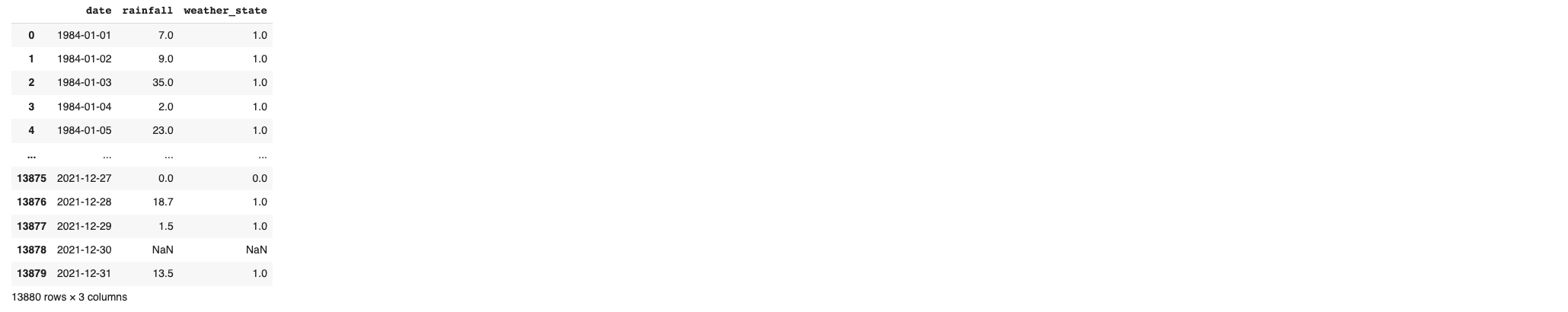
4.1.1 Rainfall categorization
In the first stage of the analysis, we import the data and categorize whether the day is rainy (value = 1) or sunny (value = 0).
Above code will produce output previews like below.
4.1.2 Function for transition probabilities order 2
This step explain the process to calculate the transition probabilities of weather states from one day to the next, considering the weather states of the previous two days, based on historical weather data. The weather states are represented as binary values: 0 for “Sunny” and 1 for “Rain”. The transition probabilities are calculated for eight different scenarios:
- P000: The probability that today is Sunny given that the day before yesterday was Sunny and yesterday was Sunny.
- P010: The probability that today is Sunny given that the day before yesterday was Sunny and yesterday was Rain.
- P100: The probability that today is Sunny given that the day before yesterday was Rain and yesterday was Sunny.
- P110: The probability that today is Sunny given that the day before yesterday was Rain and yesterday was Rain.
- P001: The probability that today is Rain given that the day before yesterday was Sunny and yesterday was Sunny.
- P101: The probability that today is Rain given that the day before yesterday was Sunny and yesterday was Rain.
- P011: The probability that today is Rain given that the day before yesterday was Rain and yesterday was Sunny.
- P111: The probability that today is Rain given that the day before yesterday was Rain and yesterday was Rain.
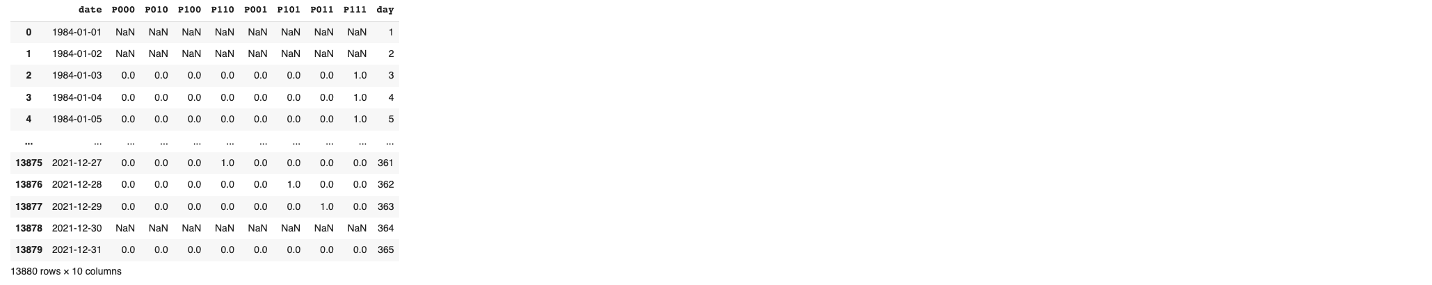
The given code defines a function calculate_transition_probabilities_orders_2_long that calculates transition probabilities based on weather conditions in a DataFrame (df). The function takes three conditions (condition1, condition2, and result) and checks if these conditions are met in consecutive rows of the DataFrame. It creates a new column with binary values indicating the occurrence of the specified conditions. NaN values are set for rows with missing data. The code then defines a list of conditions and results and iterates over them to calculate transition probabilities for each scenario. The resulting probabilities are stored in new columns in the DataFrame. The DataFrame is restructured and saved as a CSV file. Finally, the program prints ‘Completed!’ and displays a preview of the DataFrame.
Above code will produce output previews like below.
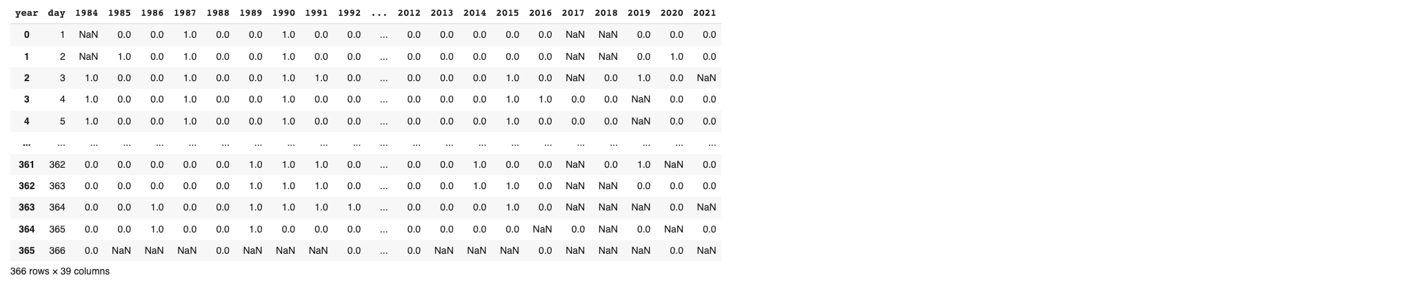
4.1.3 Reshape the data
The provided code segment executes a series of steps to transform weather data from long to wide format, to make easy for further process.
Firstly, it generates a list of unique scenarios represented by “P” values. Subsequently, a ‘year’ column is added to the DataFrame bin_df based on the ‘date’ information. The code then iterates through each unique “P” value. For each iteration, it selects the relevant columns (‘year’, ‘day’, and the current “P” value) from bin_df while removing rows with missing values. The “P” column is renamed as ‘value’. The DataFrame is then pivoted, organizing the data with ‘day’ as the index, ‘year’ as the columns, and ‘value’ as the values. Each resulting pivoted DataFrame is saved as a CSV file, with the file name corresponding to the current “P” value.
Above code will produce output previews like below.
4.1.4 Calculate number of event
This code below is responsible for calculating the total number of occurrences per day for each of the eight possible weather state transitions (P000, P001, P010, P100, P110, P101, P011, P111) over the entire period of the dataset.
In this context, each weather state transition represents a sequence of three consecutive days. For example, P010 represents a sequence where it was sunny two days ago, rained yesterday, and is sunny today. The weather states are represented as binary values: 0 for “Sunny” and 1 for “Rain”.
The code first calculates the total number of occurrences per day for each weather state transition by summing up the values in the respective columns of the binary DataFrame (bin_bin_reshape_dfxxx). It then creates a new DataFrame (num_df) that includes these totals along with the corresponding day. This DataFrame provides a daily summary of the weather state transitions for the entire period of the dataset.
Finally, the code saves this DataFrame to a CSV file for further analysis and previews the data. This step is crucial as it allows for the inspection of the calculated totals and ensures the data is correctly processed and ready for the next steps of the analysis.
Above code will produce output previews like below.

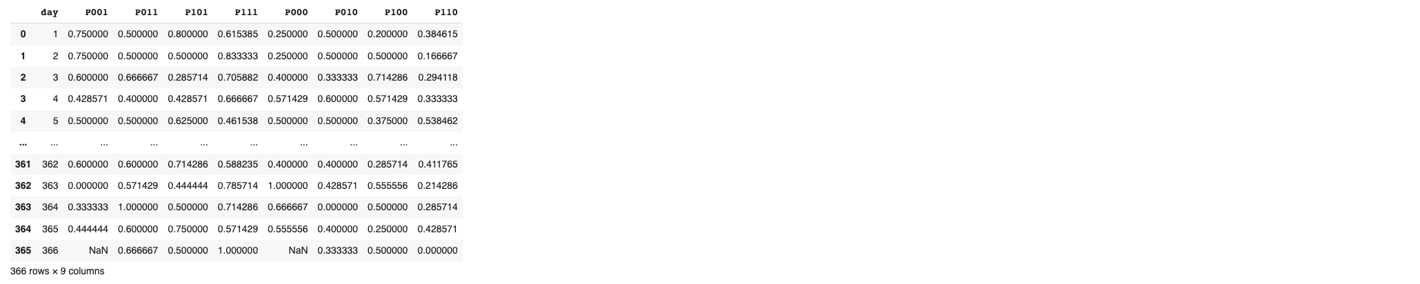
4.1.5 Calculate the probabilities
This specific code block calculates the transition probabilities for each of the four possible weather state transitions where the current day is rainy (P001, P011, P101, P111) and another four where the current day is sunny (P000, P010, P110, P100).
The transition probabilities are calculated by dividing the total number of occurrences of each rainy/sunny weather state transition by the total number of occurrences of both the rainy and sunny weather state transitions for the same previous two days. For example, the transition probability P011 is calculated by dividing the total number of P011 occurrences by the sum of the total number of P011 and P010 occurrences.
The calculated transition probabilities are then stored in a new DataFrame (prob_df_xxxx), which also includes the corresponding day. This DataFrame provides a daily summary of the transition probabilities for the entire period of the dataset.
Finally, the code saves this DataFrame to a CSV file for further analysis and previews the data. This step is crucial as it allows for the inspection of the calculated probabilities and ensures the data is correctly processed and ready for the next steps of the analysis.
Above code will produce output previews like below.
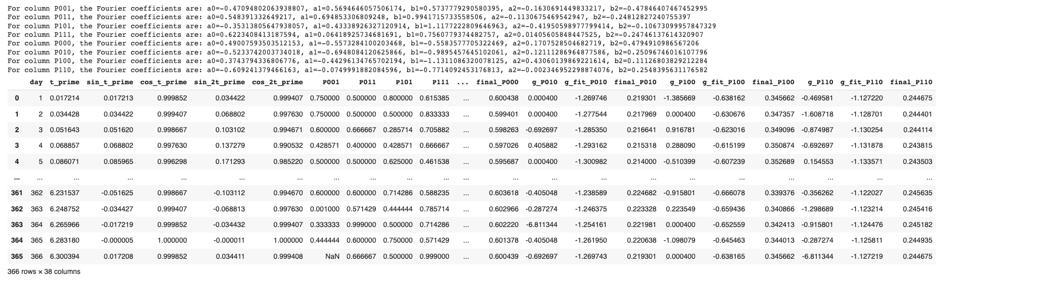
4.1.6 Converting to logit function and transform back to probability value
The code calculates Fourier coefficients and applies a logit transformation to the probability values in a pandas DataFrame prob_df. First, it modifies prob_df, replacing any instances of 0 or 1 probabilities with a small constant epsilon or 1 - epsilon respectively. This prevents errors when applying logarithms and exponentials later in the process. The script then calculates a set of variables based on the day of the year, including trigonometric functions sin_t_prime, cos_t_prime, sin_2t_prime, and cos_2t_prime based on the day of the year scaled by 2*pi/365 to reflect the cyclical nature of the calendar.
After that, the script computes the logit of the probabilities, g_a_df, which is the log of the odds ratio (i.e., the ratio of the probability of an event occurring to the probability of it not occurring). Fourier coefficients are calculated for each original column in prob_df. The Fourier series is a way to represent a function as a sum of periodic components, and in this context, it’s used to capture the cyclical patterns of the probabilities throughout the year.
Finally, the script constructs a new DataFrame result_df that includes the original probabilities, the calculated g_a_df values, fitted g_fit values (based on the Fourier series representation), and final probabilities (the inverse logit of g_a_df). This DataFrame is saved to a CSV file and then returned for review.
Above code will produce output previews like below.
4.1.7 Visualize the calculated logit and their fitted
The script visualizes the calculated logit (g) values and their fitted counterparts (g_fit) from the result_df DataFrame for both rainy and sunny day scenarios.
This is accomplished by setting up a 2-row, 4-column grid of subplots. In the first row, it plots the rainy day scenarios (P_types_rainy) and in the second row, it plots the sunny day scenarios (P_types_sunny). For each scenario (rainy or sunny) and each type of day (defined by P_types), it creates a scatter plot of ‘g’ values and overlays a line plot of ‘g_fit’ values over the course of the year (represented by the ‘day’ variable).
The script then labels each subplot with its respective day type and scenario, sets the x and y labels, and includes a legend indicating which points represent ‘g’ and which line represents ‘g_fit’.
Finally, it adjusts the layout for better visualization and displays the plot. This way, it helps to analyze how well the fitted values (g_fit) are approximating the calculated logit (g) values.
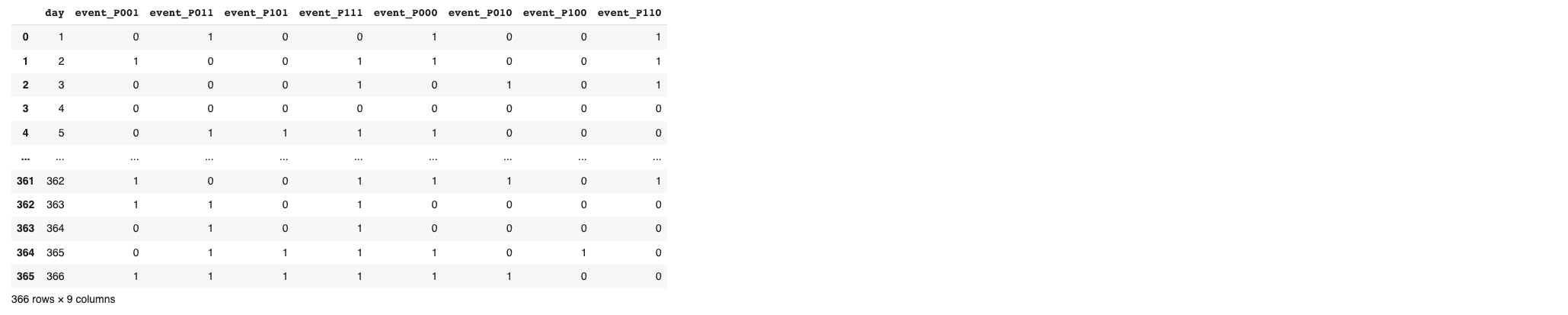
4.1.8 Generate random numbers from a uniform distribution to get the rainfall events
This code generates random numbers from a uniform distribution for each day and compares these to our probabilities to generate the events. Events are coded as 1 for rain and 0 for no rain. The new DataFrame event_df only contains the event data, with columns named event_Pxxx as specified. The data is saved in a CSV file called events.csv.
Above code will produce output previews like below.
4.1.9 Visualize the probability of rainfall occurrence
The given script produces a set of heatmaps to visualize event data related to different scenarios of rainfall given that the current day is rainy. The data, divided by months and days, represents whether it’s a rainy day (indicated by a color) or a sunny day (represented by a white block).
A heatmap is an apt choice of visualization here as it allows for an immediate visual assessment of patterns and trends in the data over a period of time (in this case, over the days of each month). Moreover, the color contrast between rainy and sunny days helps to easily distinguish between the two events. Heatmaps also excel at handling and displaying data over two dimensions (months and days, in this context), making them a clear choice for this kind of data presentation.
Firstly, the code defines different types of events (represented as ‘P_types’), the layout for the subplots, and the number of days in each month (accounting for leap years).
Then, it loops over each event type, creating a 2D array filled with NaNs to hold the event data for each day of each month. The event data is split by month and filled into this array, ensuring the correct day and month placement for each event.
Next, a heatmap for each event type is generated using seaborn, with a color scheme denoting the presence or absence of rainfall, and an outline for each day block to enhance readability. The heatmap’s axes and title are customized for each scenario.
A legend is also created to indicate the meanings of the colors in the heatmaps. The code finally adds a main title for the set of heatmaps, adjusts the layout for clear viewing, and displays the visualizations.
Before running below code, please make sure yopu already have “seaborn” installed. If not, please install it using “pip install seaborn”
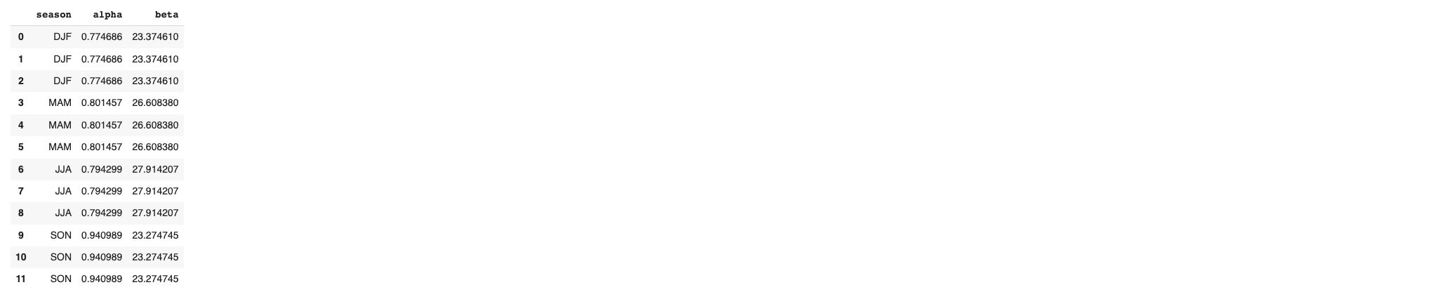
4.1.10 Gamma distribution
This code analyses a dataset of rainfall patterns. It first loads the data, and prepares it by converting the ‘date’ column into a datetime format and adding a ‘month’ column. It then assigns each entry to a season (DJF, MAM, JJA, or SON) based on the month of the year. After isolating only the rainy days, the script applies a Gamma distribution model for each season’s rainfall data. The parameters (alpha and beta) of the Gamma distribution for each season are corrected for small sample sizes using the Greenwood and Durand method. These corrected parameters are then stored in a new DataFrame, which is exported as a CSV file for future use or analysis. The resulting DataFrame provides a seasonal breakdown of the rainfall data, and offers insights into how the rainfall pattern is distributed for each season.
Above code will produce output previews like below
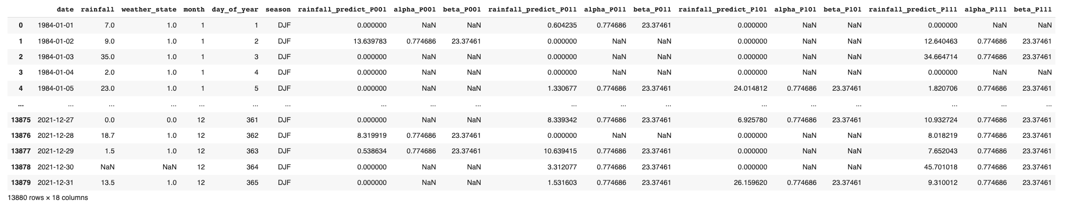
4.1.11 Generate rainfall value
Now that we have estimated the parameters for the gamma distribution for each season, and have generated event data, we can generate rainfall values based on these parameters and events.
The gamma distribution is only used to generate rainfall values for rainy days (where event = 1), as it is typically used to model positive continuous data, and cannot generate the zero values corresponding to non-rainy days.
In this script, we create a new rainfall_PXXX column for each event_PXXX column. For each season, we select the days where event_PXXX = 1, and generate rainfall values for these days using the gamma distribution with the corresponding alpha and beta parameters. These generated values are then stored in the rainfall_PXXX column. At the end, the updated DataFrame is saved to a new CSV file.
Here’s how we could do this for each P-type.
Above code will produce output previews like below.
4.2 Evaluations
Evaluating the quality of our predicted rainfall values depends on the specific goals of our analysis and the characteristics of our data. However, here are several common methods for evaluating prediction quality.
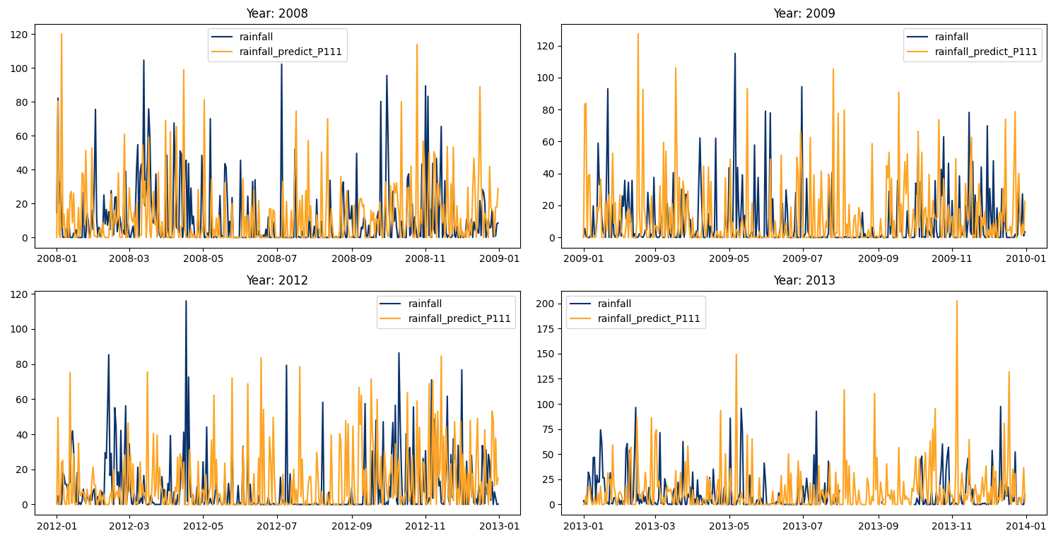
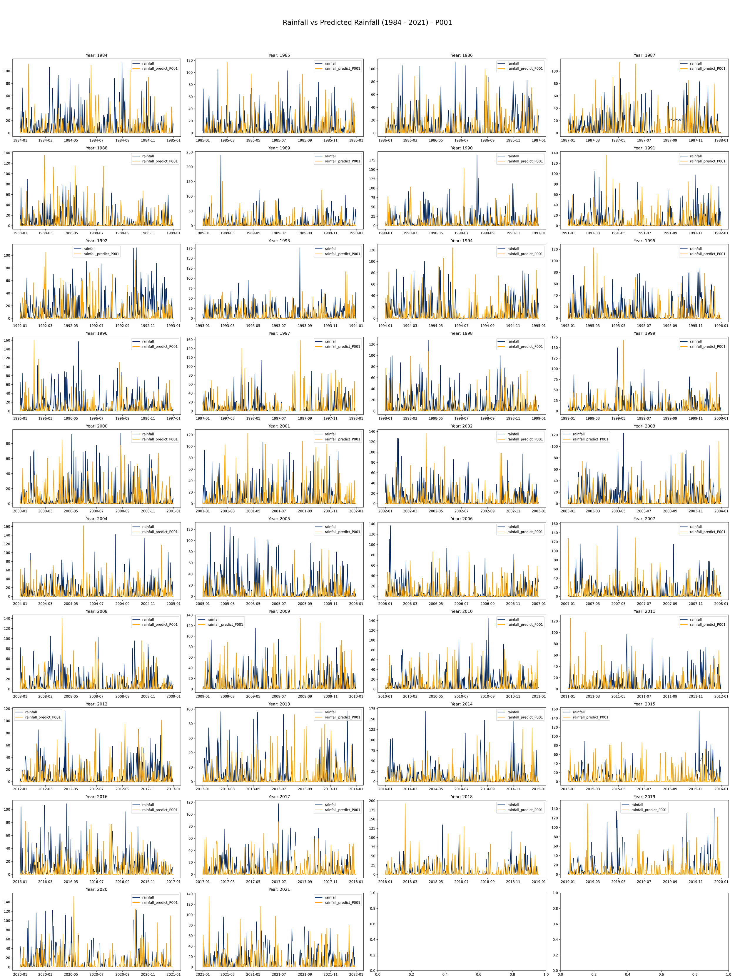
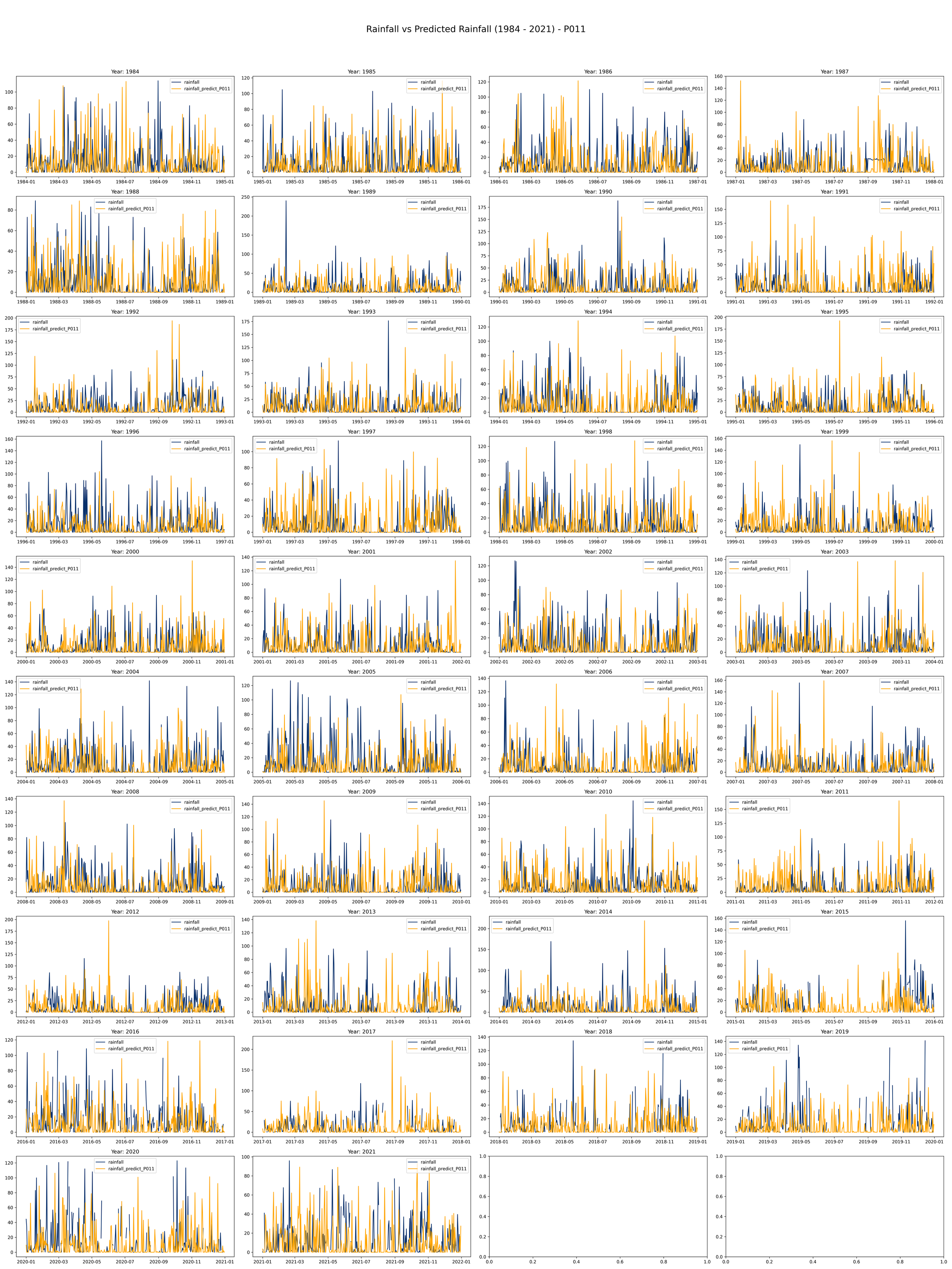
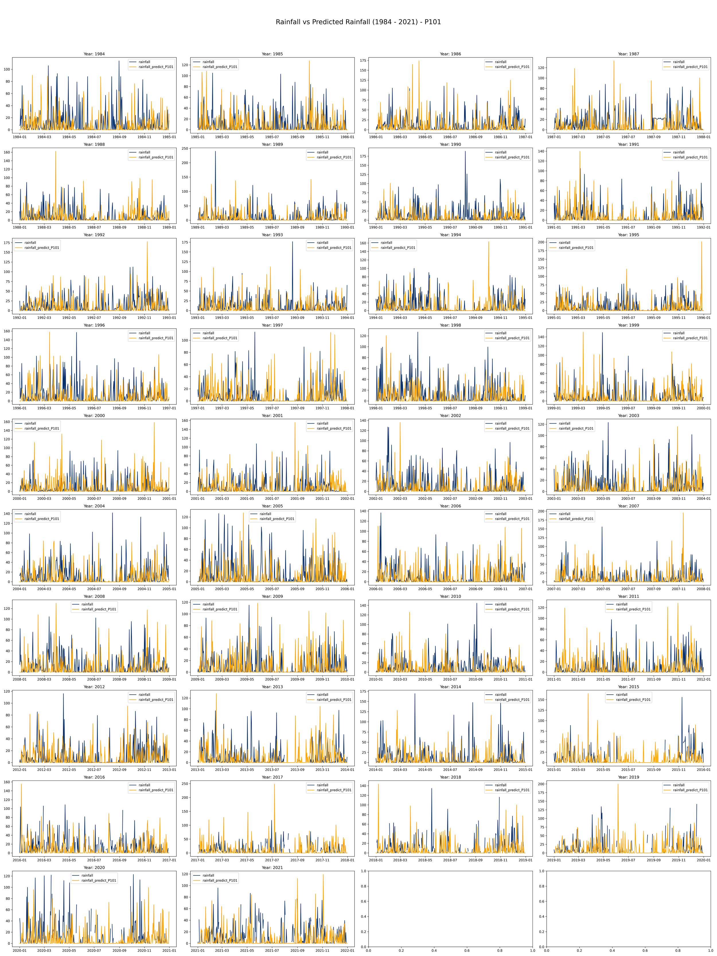
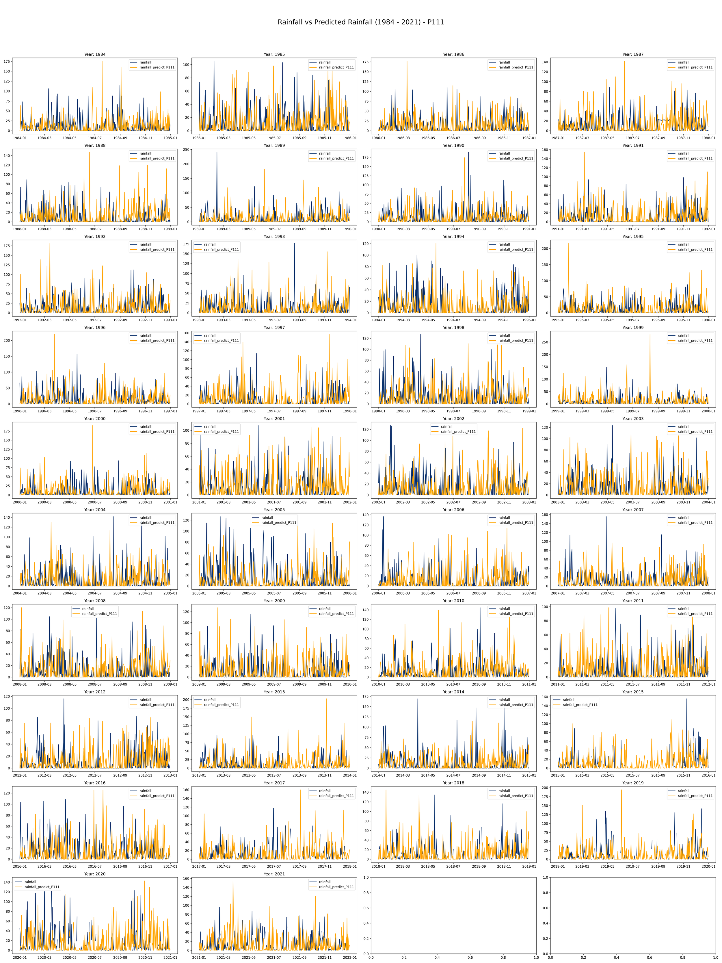
4.2.1 Visualize the rainfall compared to predicted rainfall
The given script produces a set of maps to visualize rainfall data compared to predicted rainfall different scenarios of rainfall given that the current day is rainy.
This code is meant to load, process, and plot data on annual rainfall and rainfall predictions from the years 1984 to 2021.
It initializes a plot with 10 rows and 4 columns to make room for a line plot for each year from 1984 to 2021. Each plot will compare actual rainfall (in light blue) with the predicted rainfall (in orange) over the course of a year.
4.2.2 Performance
Distribution of Errors (Residuals): We can plot a histogram or a Kernel Density Estimate plot of the residuals, which are the differences between the actual and predicted values. If our model is a good fit, the residuals should be normally distributed around zero.
Time Series of Residuals: Plotting residuals over time can show whether the errors are consistent throughout the time series, or if they vary significantly at certain time periods.
Boxplot of Errors by Year: This can help us see if the model’s performance varies significantly from year to year.
5 Results
We delve into a comprehensive analysis of rainfall prediction and its various aspects. By examining the curve adjustment chart and transforming probabilities into rainfall events, we gain insights into the predicted outcomes. Furthermore, we assess the performance of these predictions using visual comparisons, distributed errors (residuals), time series of residuals, and boxplot of error by year. This chapter aims to elucidate the accuracy and reliability of our rainfall prediction model.
5.1 Adjustment curve
The scatter plot visualizes the adjustment curve for generating daily rainfall data using Fourier regression analysis. The data spans from 1984 to 2021. Each subplot corresponds to different weather patterns, characterized by the variables ‘P001’, ‘P011’, ‘P101’, ‘P111’, ‘P000’, ‘P010’, ‘P100’, and ‘P110’.
The top row of plots shows the fitting model for rainy days (‘P001’, ‘P011’, ‘P101’, ‘P111’). Here, the patterns in the fitted models (g_fit) align with the data generated by g_a, indicating that the Fourier model accurately captures the distribution pattern of rainfall across different types of rainy day events.
The second row presents the fitting model for dry days (‘P000’, ‘P010’, ‘P100’, ‘P110’). In these plots, the peak of the dry season, occurring in the June-July-August (JJA) period, is prominently reflected in the peak of the g_fit line plot. Conversely, the rainfall is lowest during this period, which is depicted as a valley in the model.
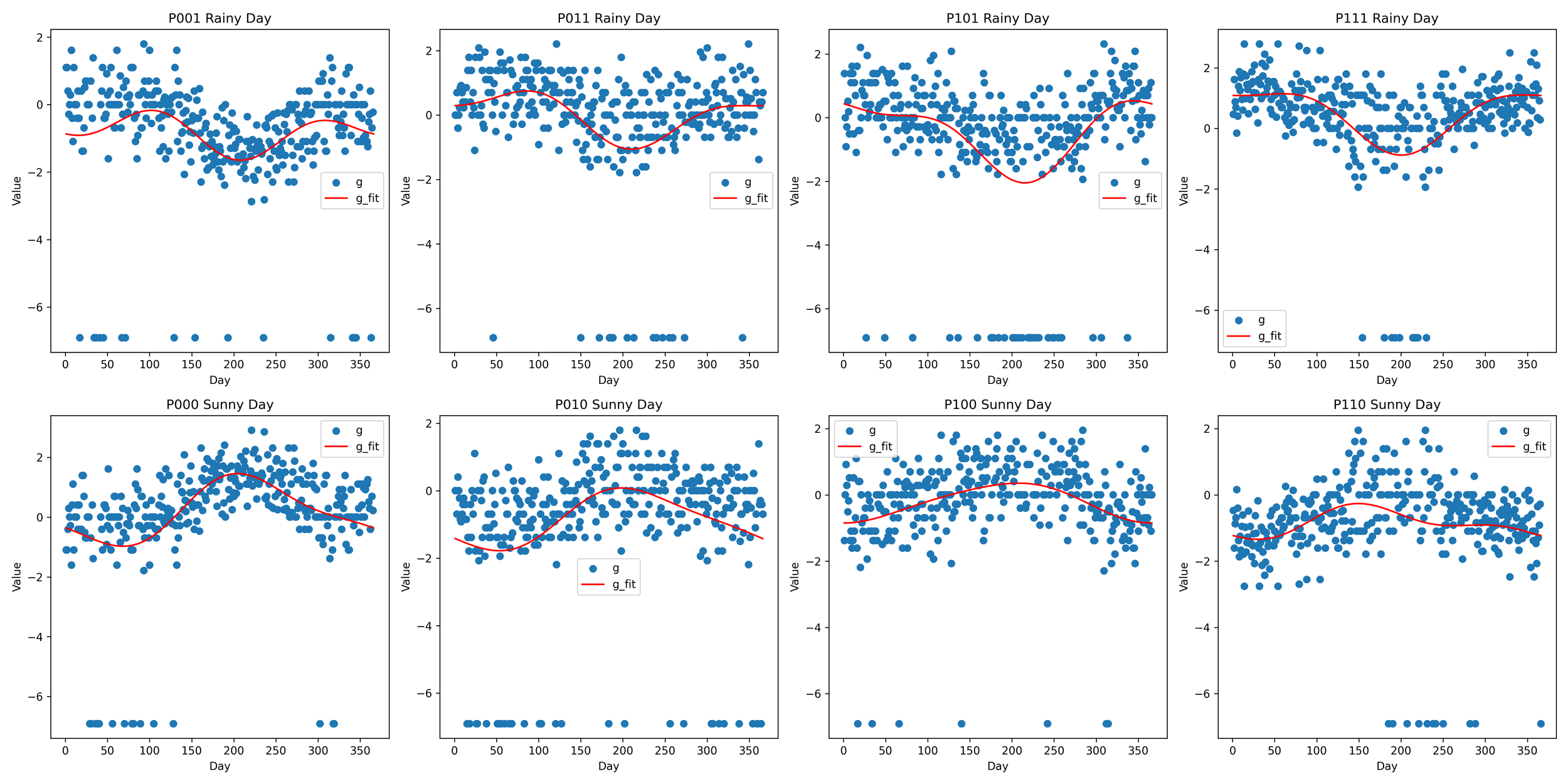
Above visualization effectively demonstrates the application and accuracy of the Fourier regression analysis in modeling and simulating daily weather patterns, both for rainy and dry conditions, over a significant period. The g_fit line plots accurately reflect the distribution patterns of the original data (g), implying that the Fourier model is a suitable tool for simulating these weather patterns.
5.2 Transforming the probability into rainfall event
The image is a set of four heatmaps, each representing a different scenario: ‘P001’, ‘P011’, ‘P101’, and ‘P111’. These scenarios are likely representative of different weather conditions or patterns. Each heatmap shows the pattern of rainfall across a year. The x-axis denotes the day of the month while the y-axis represents the month itself, ranging from 1 (January) to 12 (December).
The color intensity in each cell indicates the probability of rainfall. Darker shades symbolize a higher likelihood of rain, while lighter shades indicate a lower likelihood. This color gradient allows us to visually comprehend the variability and seasonality of rainfall across different periods of the year.
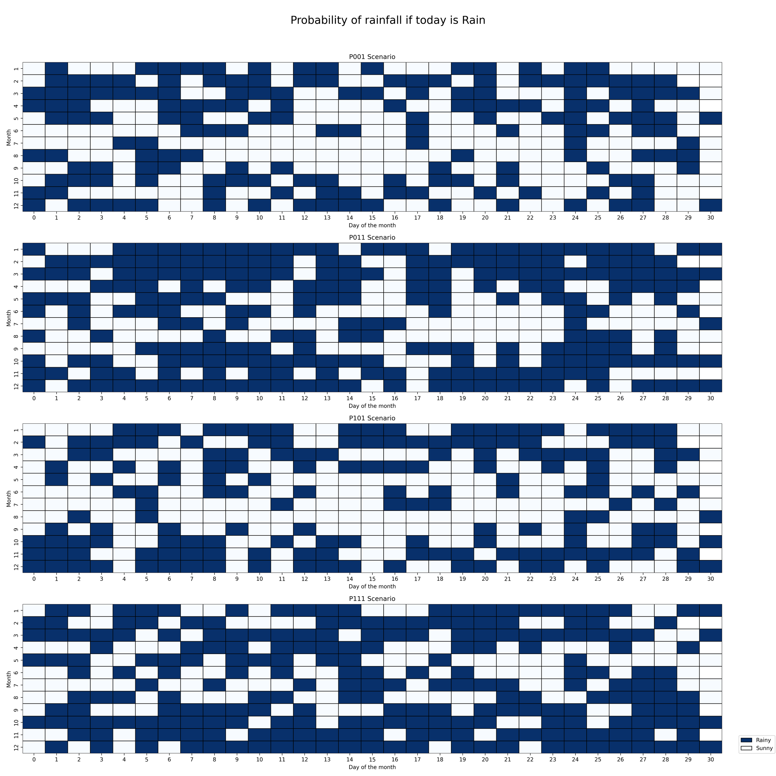
From these heatmaps, one can observe the days and months when rainfall is more or less likely, given that the day is classified as ‘rainy’. These visualizations provide an intuitive understanding of rainfall patterns and their variations throughout the year for each respective scenario.
5.3 Predicted rainfall
The daily rainfall generated by the Fourier regression model and compared with the daily observation data from the Bogor Climatology Station from 1984-2021 in the image below (example using Year 2008-200- and 2012-2013) indicates that the predicted rainfall shows rainfall values produced by the model are higher than the observation data (overrated) with a pattern that tends to be somewhat dissimilar.
5.4 Performance
Evaluating the quality of our predicted rainfall values depends on the specific goals of our analysis and the characteristics of our data. However, here are several common methods for evaluating prediction quality:
Visual comparison: It’s a plot of the predicted values against the observed values. This can give us a quick, intuitive sense of how closely our predictions match the actual values. While visually comparing the predicted and actual rainfall data is important and necessary, it is not sufficient on its own to evaluate the performance of the prediction model.
Distribution of Errors (Residuals): This plot shows the distribution of residuals (errors), which are the differences between the predicted and actual rainfall values.
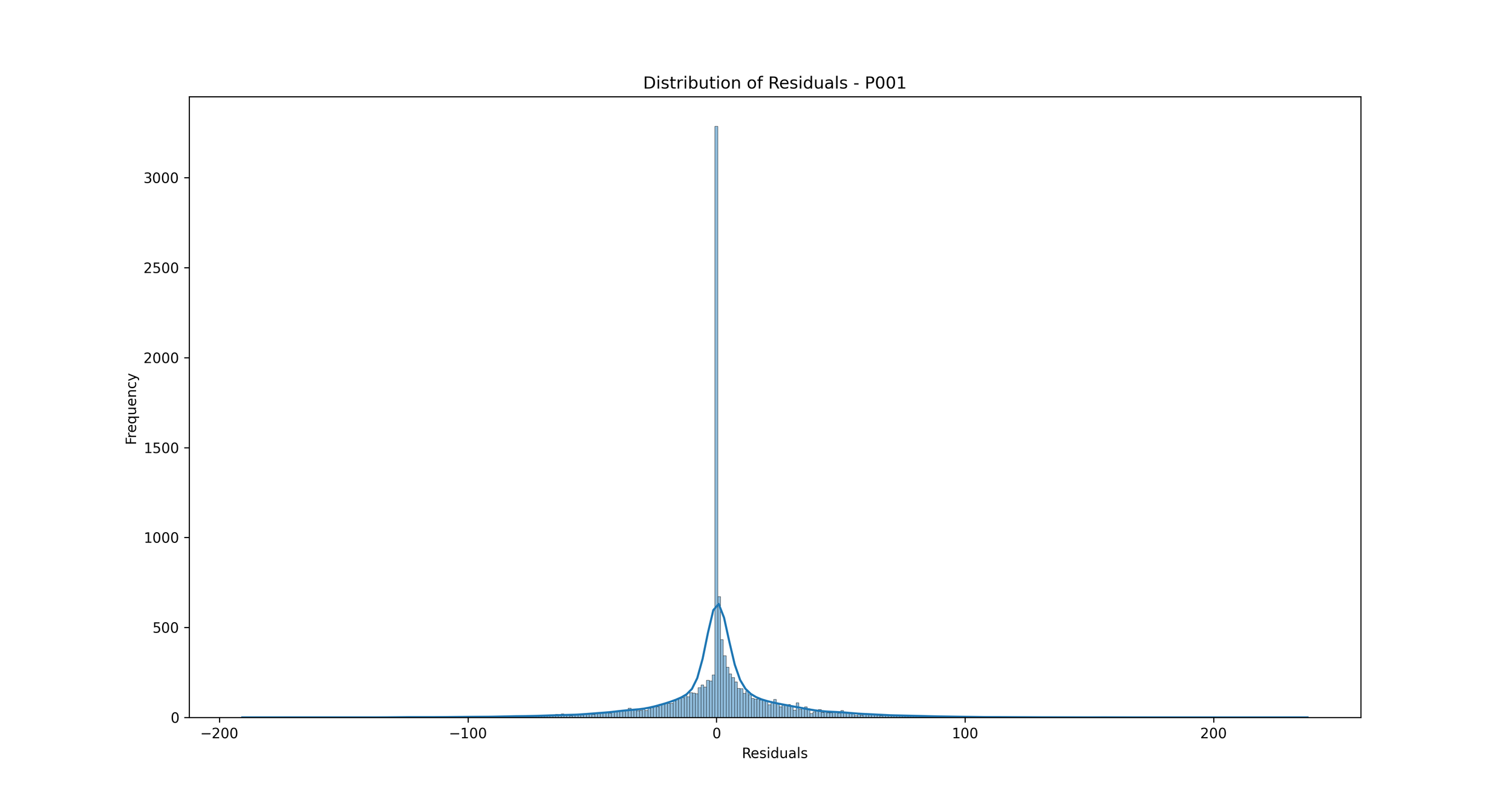
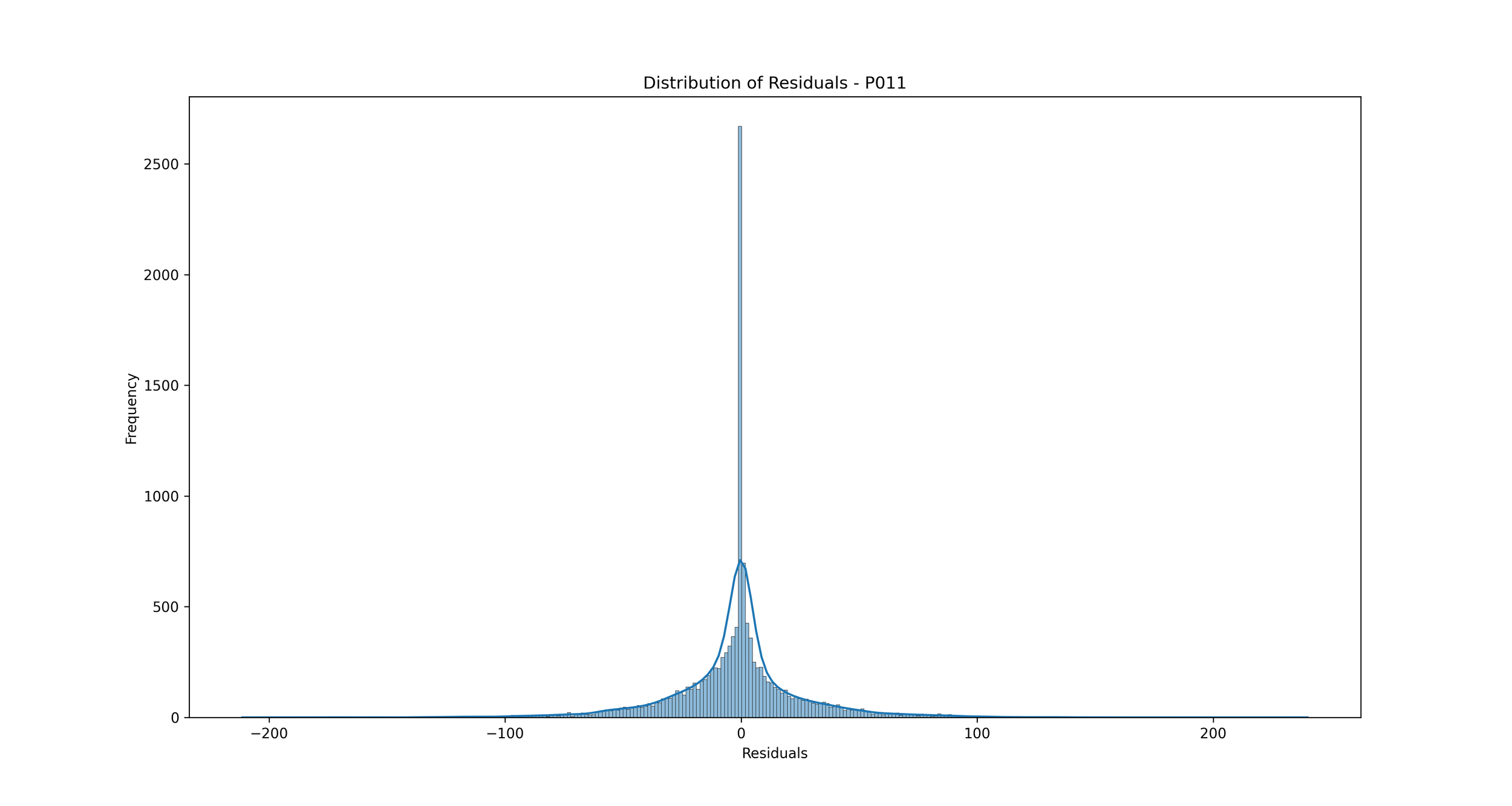
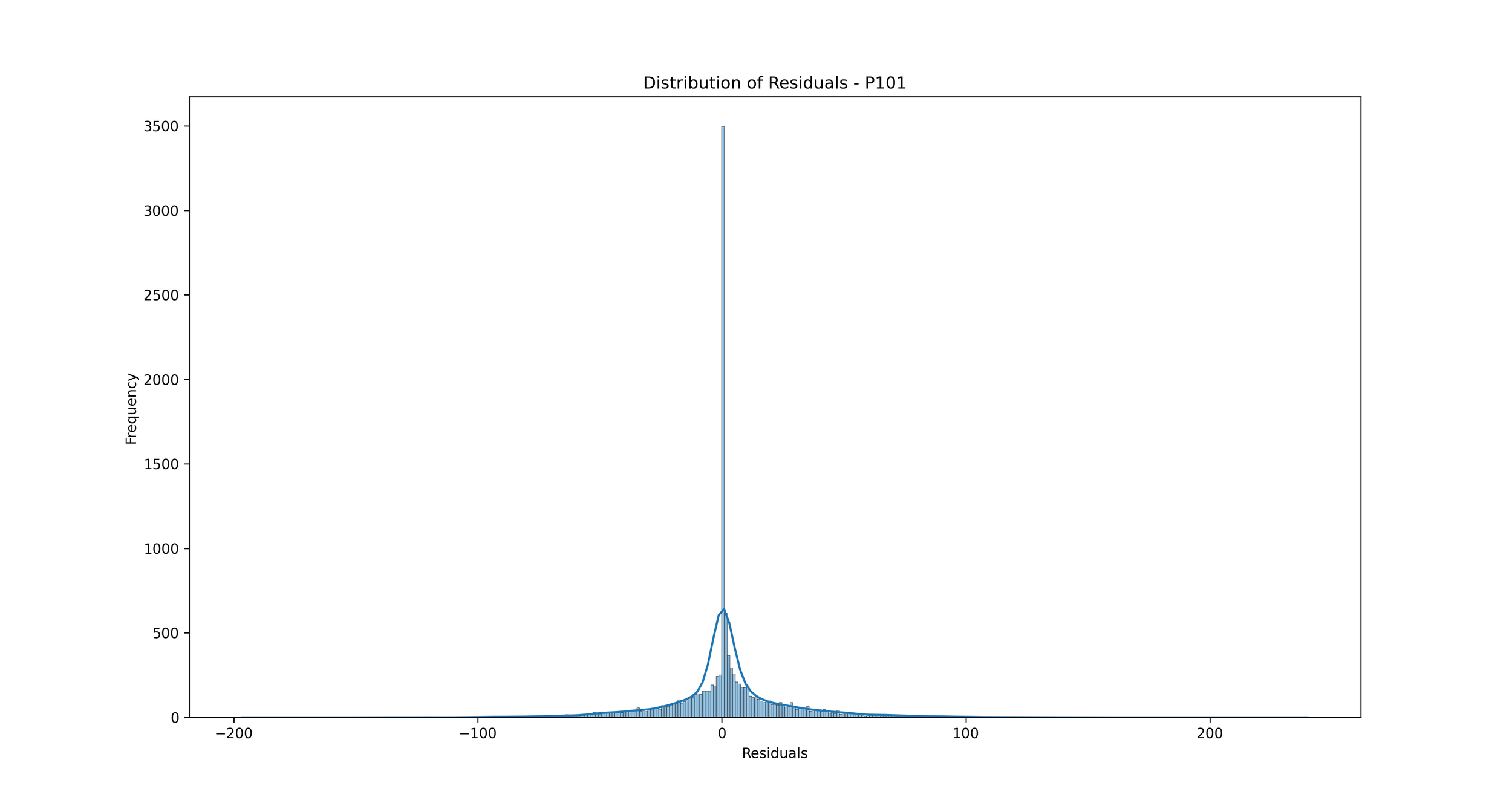
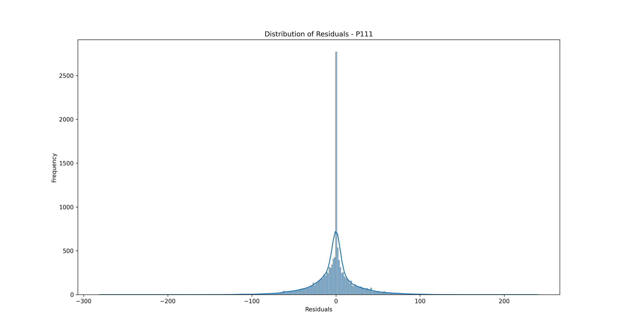
In the context of rainfall prediction, if the residuals are normally distributed and centered around zero, it indicates that your model has made errors that are random and not biased, which is a good sign. If the distribution is not centered around zero or is highly skewed, it indicates that your model may be consistently overestimating or underestimating the rainfall.
Time Series of Residuals: This plot shows how residuals change over time.
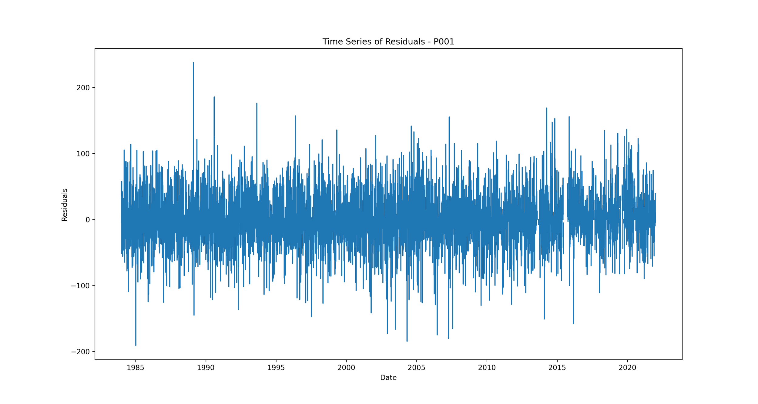
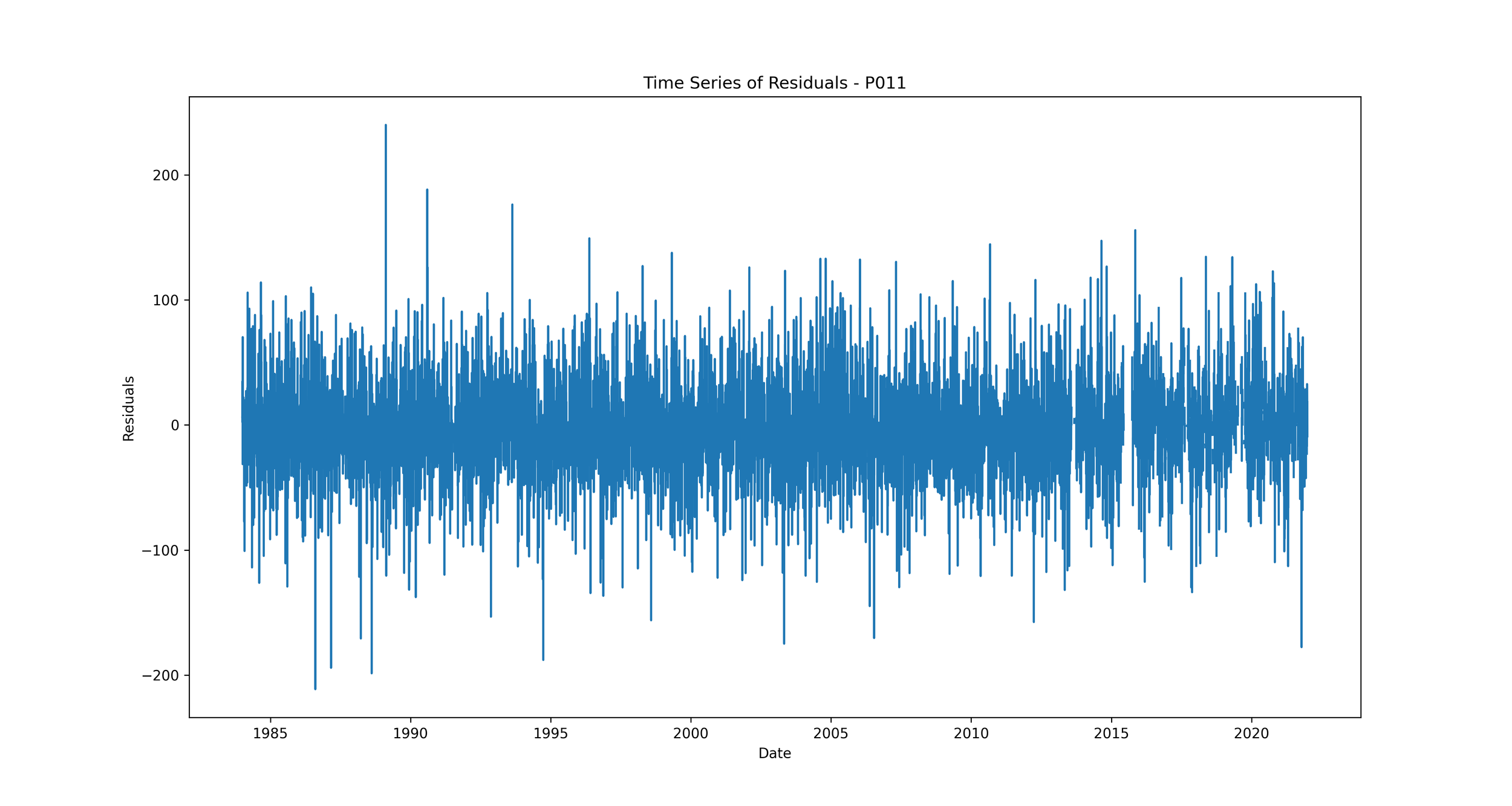
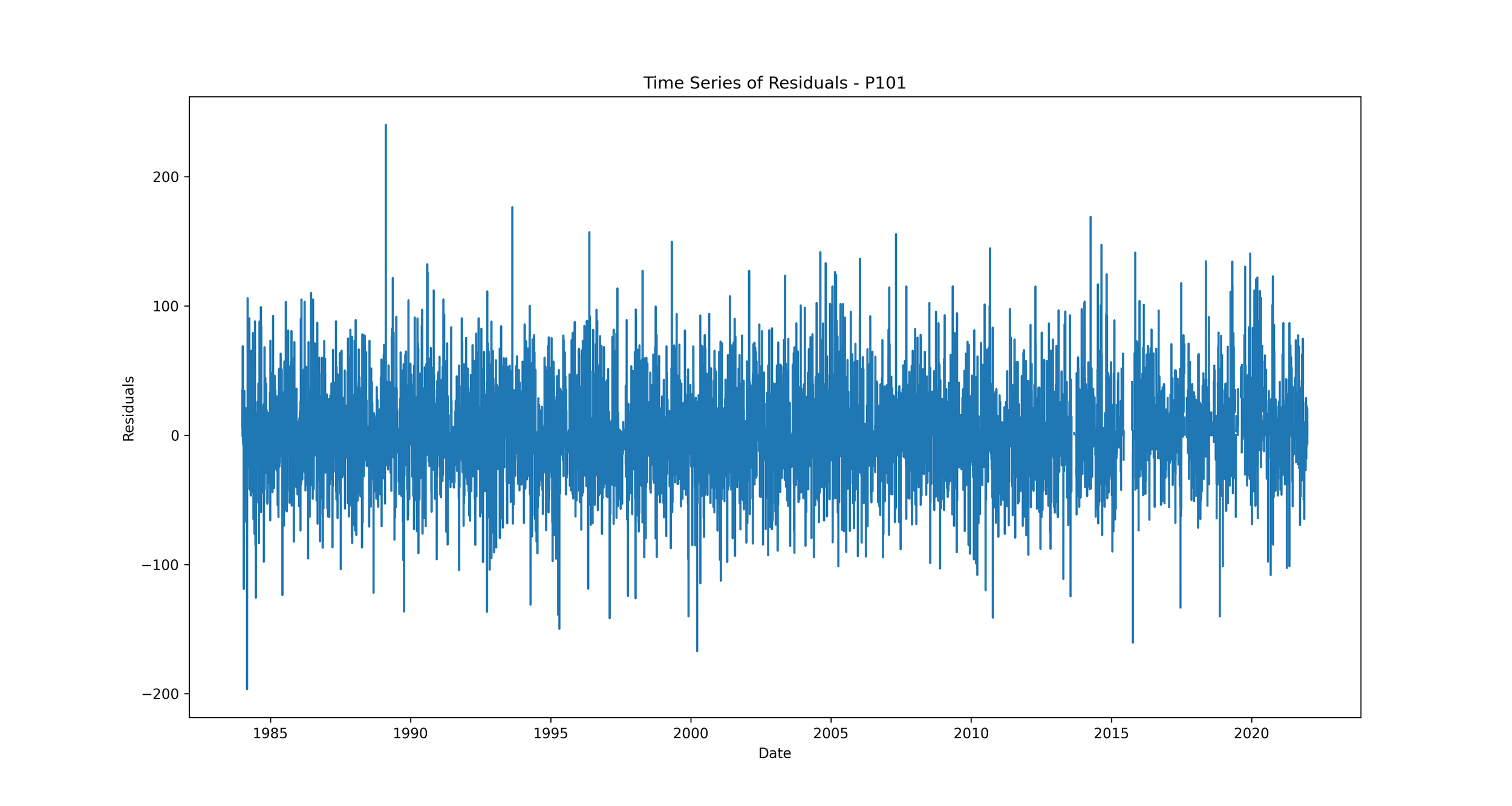
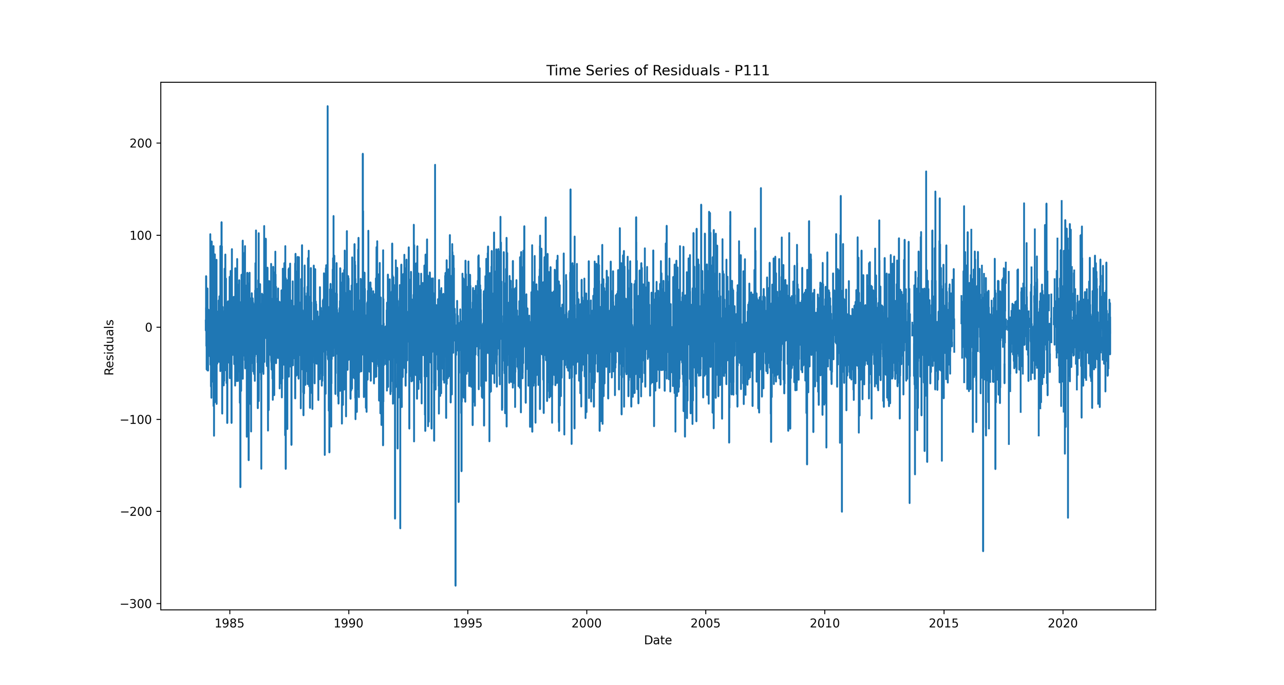
We should expect to see no clear pattern in the residuals over time. If we see patterns, such as the residuals increasing or decreasing over time, it suggests that our model is not capturing some trend in the data. This could indicate a problem with our model that needs to be addressed.
Boxplot of Error by Year: This plot shows the distribution of residuals for each year.
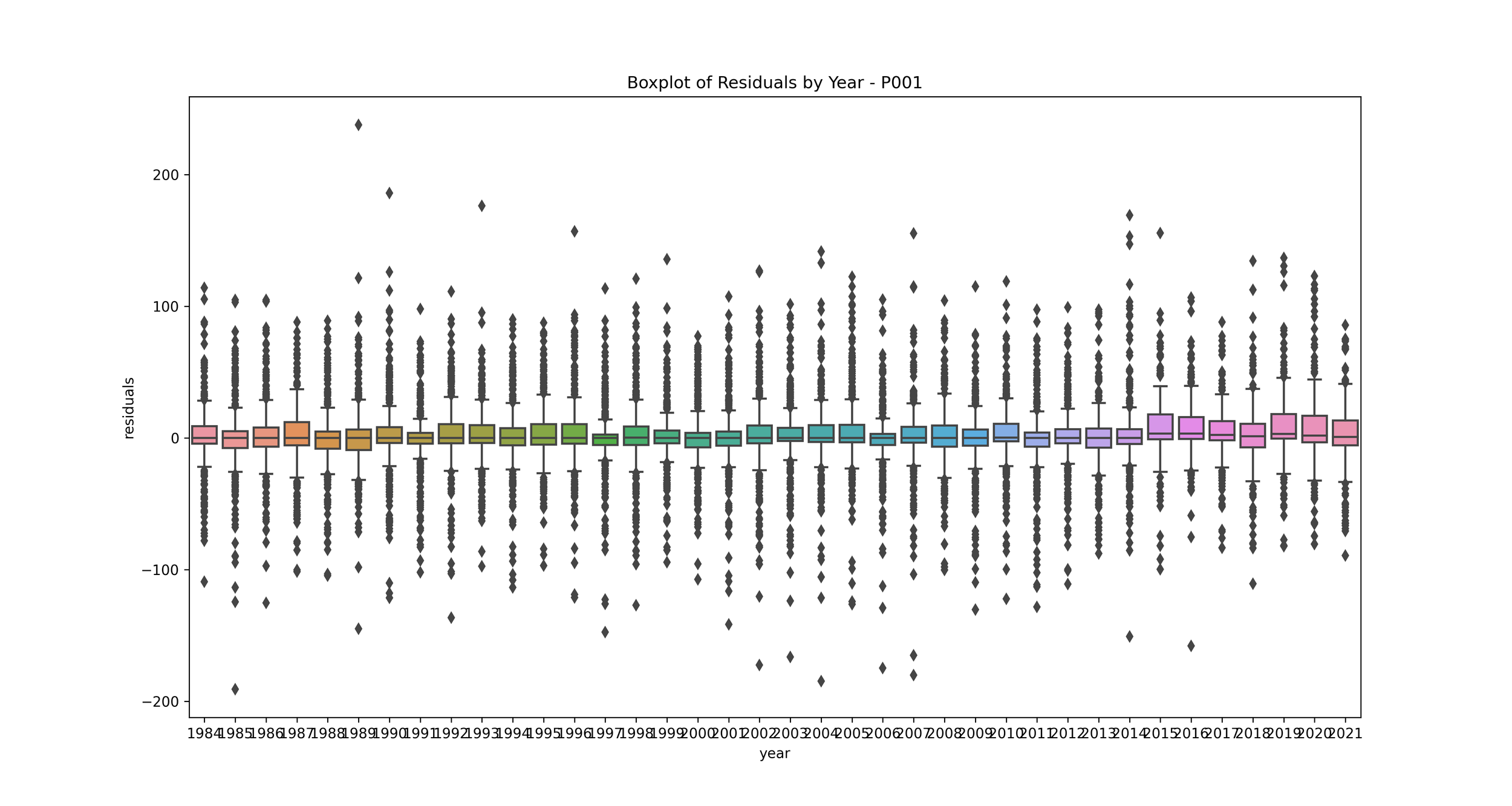
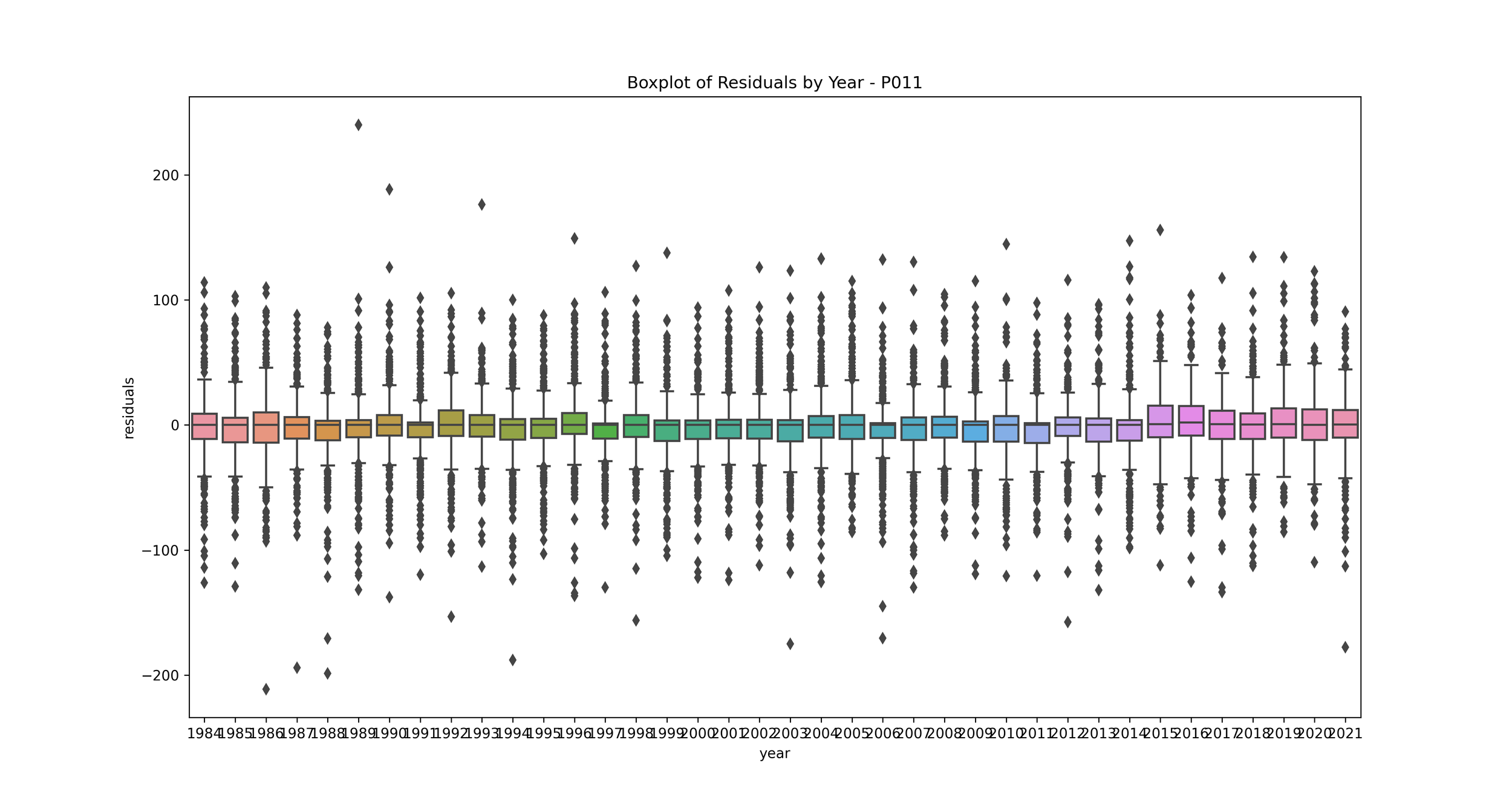
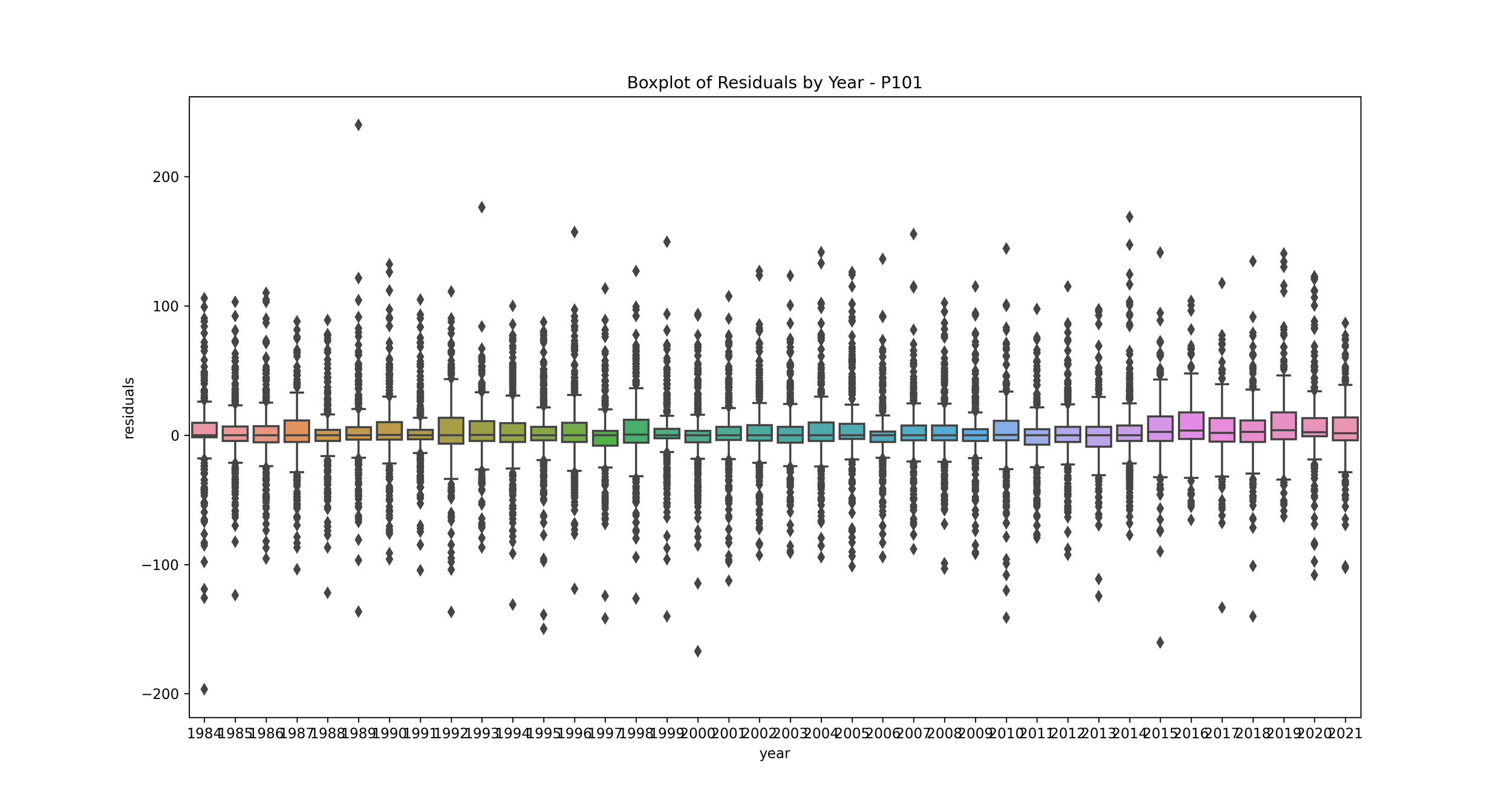
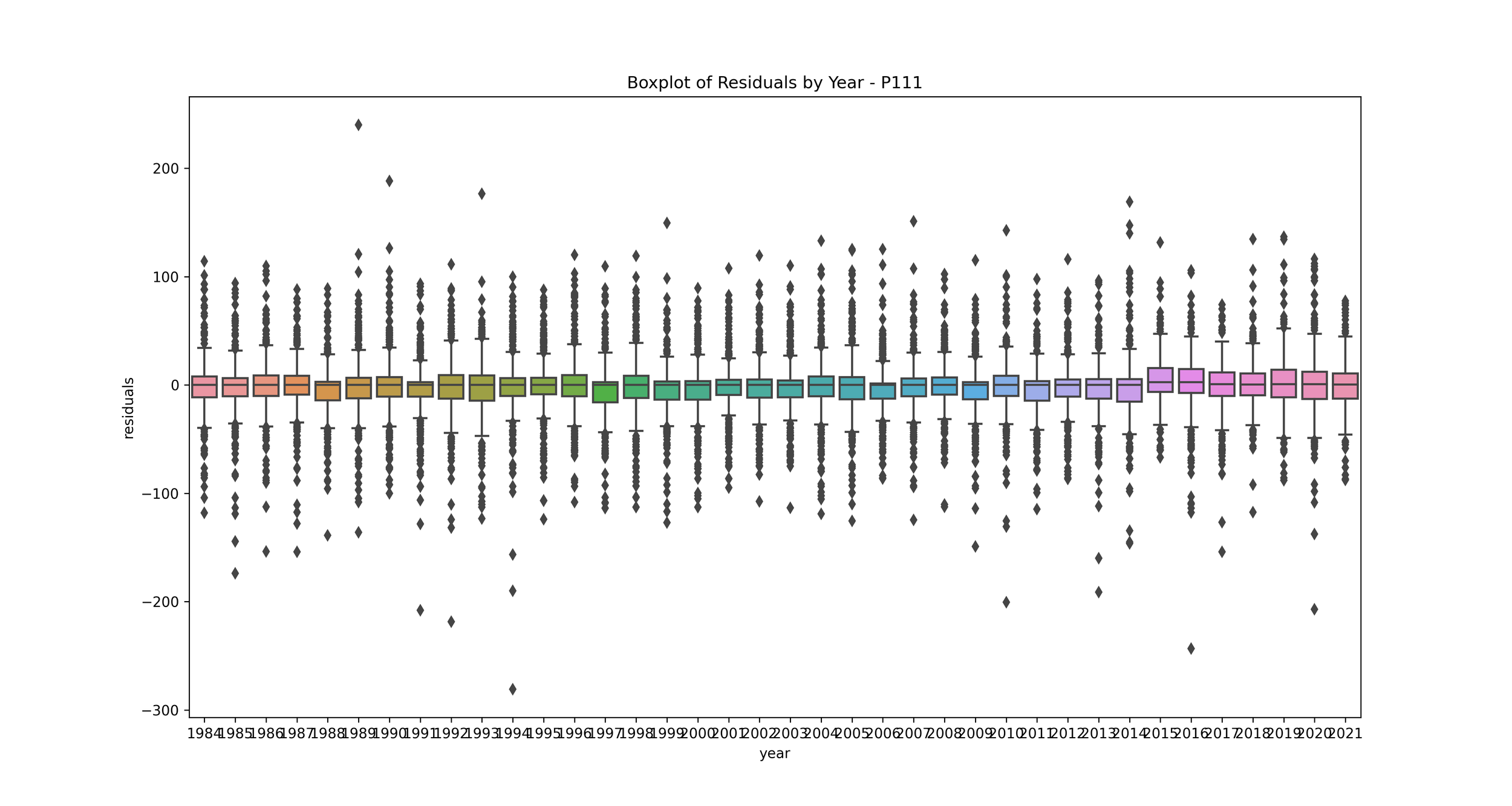
This can help you understand if your model’s performance is consistent over time. If some years have much higher or lower residuals, it may indicate that those years had unusual rainfall patterns that your model didn’t capture. You may want to investigate further to understand what’s causing these discrepancies.
6 Conclusion
Markov-chain models, when combined with Fourier regression equations and logit transformations, can be useful in estimating rainfall occurrence probabilities and generating synthetic rainfall data. This generated data can have practical applications in various fields, such as agriculture and urban planning, where accurate rainfall data is crucial for informed decision-making.
7 References
Ashley, R. M., Balmforth, D. J., Saul, A. J., & Blanskby, J. D. (2005). Flooding in the future–predicting climate change, risks and responses in urban areas. Water Science and Technology, 52(5), 265-273. https://doi.org/10.2166/WST.2005.0142
Bellone, E., Hughes, J. P., & Guttorp, P. (2000). A hidden Markov model for downscaling synoptic atmospheric patterns to precipitation amounts. Climate Research, 15(1), 1-12. https://www.jstor.org/stable/e24867295
Boer, R., Notodipuro, K.A., Las, I. 1999. Prediction of Daily Rainfall Characteristics from Monthly Climate Indices. RUT-IV report. National Research Council, Indonesia.
Cho, H., K. P. Bowman, and G. R. North. 2004. A Comparison of Gamma and Lognormal Distributions for Characterizing Satellite Rain Rates from the Tropical Rainfall Measuring Mission. J. Appl. Meteor. Climatol., 43, 1586–1597. https://doi.org/10.1175/JAM2165.1
Hughes, J. P., Guttorp, P., & Charles, S. P. (1999). A non-homogeneous hidden Markov model for precipitation occurrence. Journal of the Royal Statistical Society: Series C (Applied Statistics), 48(1), 15-30. https://doi.org/10.1111/1467-9876.00136
Rodriguez-Iturbe, I., Cox, D. R., & Isham, V. (1987). Some models for rainfall based on stochastic point processes. Proceedings of the Royal Society of London. Series A, Mathematical and Physical Sciences, 410(1839), 269-288. https://doi.org/10.1098/rspa.1987.0039
Rosenzweig, C., Tubiello, F. N., Goldberg, R., Mills, E., & Bloomfield, J. (2002). Increased crop damage in the US from excess precipitation under climate change. Global Environmental Change, 12(3), 197-202. https://doi.org/10.1016/S0959-3780(02)00008-0
Srikanthan, R., & McMahon, T. A. (2001). Stochastic generation of annual, monthly and daily climate data: A review. Hydrology and Earth System Sciences Discussions, 5(4), 653-670. https://doi.org/10.5194/hess-5-653-2001
Stern, R. D., & Coe, R. (1984). A model fitting analysis of daily rainfall data. Journal of the Royal Statistical Society. Series A (General), 147(1), 1-34. https://doi.org/10.2307/2981736
VanTassell, L.W., J.W. Richardson and J.R. Conner. 1990. Simulation of meteorological data for use in agricultural production studies. Agric. System 34:319-336. https://doi.org/10.1016/0308-521X(90)90011-E
Waggoner, P.E. (1989). Anticipating the frequency distribution of precipitation if climate change alters its mean. Agric. For. Meteor. 47:321-337. https://doi.org/10.1016/0168-1923(89)90103-2
Wilks, D. S. (1990). Maximum likelihood estimation for the gamma distribution using data containing zeros. Journal of Climate, 3(12), 1495-1501. https://doi.org/10.1175/1520-0442(1990)003%3C1495:MLEFTG%3E2.0.CO;2
Wilks, D. S. (1998). Multisite generalization of a daily stochastic precipitation generation model. Journal of Hydrology, 210(1-4), 178-191. https://doi.org/10.1016/S0022-1694(98)00186-3
Wilks, D. S. (2011). Statistical methods in the atmospheric sciences (Vol. 100). Academic press. https://doi.org/10.1016/C2017-0-03921-6